Download
1 / 36
360 likes | 364 Views
EE255/CPS226 Continuous Random Variables. Dept. of Electrical & Computer engineering Duke University Email: bbm@ee.duke.edu , kst@ee.duke.edu. Definitions. Distribution function: If F X (x) is a continuous function of x, then X is a continuous random variable.

E N D
EE255/CPS226Continuous Random Variables Dept. of Electrical & Computer engineering Duke University Email: bbm@ee.duke.edu, kst@ee.duke.edu
Definitions • Distribution function: • If FX(x) is a continuous function of x, then X is a continuous random variable. • FX(x): discrete in x Discrete rv’s • FX(x): piecewise continuous Mixed rv’s Bharat B. Madan, Department of Electrical and Computer Engineering, Duke University
Probability Density Function (pdf) • X : continuous rv, then, • pdf properties: Bharat B. Madan, Department of Electrical and Computer Engineering, Duke University
Exponential Distribution • Arises commonly in reliability & queuing theory. • It exhibits memory-less (Markov) property. • Related to Poisson distribution • Inter-arrival time between two IP packets (or voice calls) • Time interval between failures, etc. • Mathematically, Bharat B. Madan, Department of Electrical and Computer Engineering, Duke University
Exp Distribution: Memory-less Property • A light bulb is replaced only after it has failed. • Conversely, a critical space shuttle component is replaced after some fixed no. of hours of use. Thus exhibiting memory property. • Wait time in a queue at the check-in counter? • Exp( ) distribution exhibits the useful memory-less property, i.e. the future occurrence of random event (following Exp( ) distribution) is independent of when it occurred last. Bharat B. Madan, Department of Electrical and Computer Engineering, Duke University
Memory-less Property (contd.) • Assuming rv X follows Exp( ) distribution, • Memory-less property: find P( ) at a future point. • X > u, is the life time, y is the residual life time Bharat B. Madan, Department of Electrical and Computer Engineering, Duke University
Memory-less Property (contd.) • Memory-less property • If the component’s life time is exponentially distributed, then, • The remaining life time does not depend on how long it has already working. • If inter-arrival times (between calls) are exponentially distributed, then, time we need still wait for a new arrival is independent of how long we have already waited. • Memory-less property a.k.a Markov property • Converse is also true, i.e. if X satisfies Markov property, then it must follow Exp() distribution. Bharat B. Madan, Department of Electrical and Computer Engineering, Duke University
Reliability & Failure Rate Theory • Reliability R(t): failure occurs after time ‘t’. Let X be the life time of a component subject to failures. • N0: total components (fixed); Ns: survived ones • f(t)Δt : unconditional prob(fail) in the interval (t, t+Δt] • conditional failure prob.? Bharat B. Madan, Department of Electrical and Computer Engineering, Duke University
Reliability & Failure Rate Theory (contd.) • Instantaneous failure rate: h(t) (#failures/10k hrs) • Let f(t) (failure density fn) be EXP( λ). Then, • Using simple calculus, Bharat B. Madan, Department of Electrical and Computer Engineering, Duke University
Failure Behaviors • There are other failure density functions that can be used to model DFR, IFR (or mixed) failure behavior DFR IFR CFR Failure rate Time • DFR phase: Initial design, constant bug fixes • CFR phase: Normal operational phase • IFR phase: Aging behavior Bharat B. Madan, Department of Electrical and Computer Engineering, Duke University
HypoExponential • HypoExp: multiple Exp stages. • 2-stage HypoExp denoted as HYPO(λ1, λ2). The density, distribution and hazard rate function are: • HypoExp results in IFR: 0 min(λ1, λ2) Bharat B. Madan, Department of Electrical and Computer Engineering, Duke University
Erlang Distribution • Special case of HypoExp: All r stages are identical. • [X > t] = [Nt < r] (Nt: no. of stresses applied in (0,t] and Nt is Possion (param λt). This interpretation gives, Bharat B. Madan, Department of Electrical and Computer Engineering, Duke University
Gamma Distribution • Gamma density function is, • Gamma distribution can capture all three failure models, viz. DFR, CFR and IFR. • α = 1: CFR • α <1 : DFR • α >1 : IFR Bharat B. Madan, Department of Electrical and Computer Engineering, Duke University
HyperExponential Distribution • Hypo or Erlang Sequential Exp( ) stages. • Parallel Exp( ) stages HyperExponential. • Sum of k Exp( ) also gives k-stage HyperExp • CPU service time may be modeled as HyperExp Bharat B. Madan, Department of Electrical and Computer Engineering, Duke University
Weibull Distribution • Frequently used to model fatigue failure, ball bearing failure etc. (very long tails) • Weibull distribution is also capable of modeling DFR (α < 1), CFR (α = 1) and IFR (α >1). • α is called the shape parameter. Bharat B. Madan, Department of Electrical and Computer Engineering, Duke University
Log-logistic Distribution • Log-logistic can model DFR, CFR and IFR failure models simultaneously, unlike previous ones. • For, κ > 1, the failure rate first increases with t (IFR); after momentarily leveling off (CFR), it decreases (DFR) with time, all within the same distribution. Bharat B. Madan, Department of Electrical and Computer Engineering, Duke University
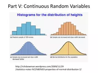
Gaussian (Normal) Distribution • Bell shaped – intuitively pleasing! • Central Limit Theorem: mean of a large number of mutually independent rv’s (having arbitrary distributions) starts following Normal distribution as n • μ: mean, σ: std. deviation, σ2: variance (N(μ, σ2)) • μ and σ completely describe the statistics. This is significant in statistical estimation/signal processing/communication theory etc. Bharat B. Madan, Department of Electrical and Computer Engineering, Duke University
Normal Distribution (contd.) • N(0,1) is called normalized Guassian. • N(0,1) is symmetric i.e. • f(x)=f(-x) • F(z) = 1-F(z). • Failure rate h(t) follows IFR behavior. • Hence, N( ) is suitable for modeling long-term wear or aging related failure phenomena. Bharat B. Madan, Department of Electrical and Computer Engineering, Duke University
Uniform Distribution • U(a,b) constant over the (a,b) interval Bharat B. Madan, Department of Electrical and Computer Engineering, Duke University
Defective Distributions • If • Example: Bharat B. Madan, Department of Electrical and Computer Engineering, Duke University
Functions of Random Variables • Often, rv’s need to be transformed/operated upon. • Y = Φ (X) : so, what is the distribution of Y ? • Example: Y = X2 • If fX(x) is N(0,1), then, • Above fY(y) is also known as the χ2 distribution (with 1-d of freedom). Bharat B. Madan, Department of Electrical and Computer Engineering, Duke University
Functions of R V’s (contd.) • If X is uniformly distributed, then, Y= -λ-1ln(1-X) follows Exp( ) distribution • transformations may be used to synthetically generate random numbers with desired distributions. • Computer Random No. generators may employ this method. Bharat B. Madan, Department of Electrical and Computer Engineering, Duke University
Functions of R V’s (contd.) • Given, • A monotone differentiable function, • Above method suggests a way to get the desired CDF, given some other simple type of CDF. This allows generation of random variables with desired distribution. • Choose Φ to be F. • Since, Y=F(X), FY(y) = y and Y is U(0,1). • To generate a random variable with X having desired distribution, choose generate U(0,1) random variable Y, then transform y to x= F-1(y) . Bharat B. Madan, Department of Electrical and Computer Engineering, Duke University
Jointly Distributed RVs • Joint Distribution Function: • Independent rv’s: iff the following holds: Bharat B. Madan, Department of Electrical and Computer Engineering, Duke University
Joint Distribution Properties Bharat B. Madan, Department of Electrical and Computer Engineering, Duke University
Joint Distribution Properties (contd) Bharat B. Madan, Department of Electrical and Computer Engineering, Duke University
Order Statistics (min, max function) • Define Yk ( known as the kth order statistics) • Y1 = min{X1, X2, …, Xn} • Yn = max{X1, X2, …, Xn} • Permute {Xi} so that {Yi} are sorted (ascending order) • Y1 : life of a system with ‘series’ of components. • Yn : with ‘parallel’ (redundant) set of components. • Distribution of Yk ? • Prob. that exactly j of Xi values are in (-∞,y] and remaining (n-j) values in (y, ∞] is: Bharat B. Madan, Department of Electrical and Computer Engineering, Duke University
Sorted random sequence Yk Observe that there are at least k Xi’s that are<= y. Some of the remaining Xi’s may Also be <= y Bharat B. Madan, Department of Electrical and Computer Engineering, Duke University
Sorted RV’s (contd) • Using FY(y), reliability may be computed as, • In general, Bharat B. Madan, Department of Electrical and Computer Engineering, Duke University
Sorted RV’s: min case (contd) • ith component’s life time: EXP(λi), then, • Hence, life time for such a system also has EXP() distribution with, • For the parallel case, the resulting distribution is not EXP( ) Bharat B. Madan, Department of Electrical and Computer Engineering, Duke University
Sum of Random Variables • Z = Φ(X, Y) ((X, Y) may not be independent) • For the special case, Z = X + Y • The resulting pdf is, • Convolution integral Bharat B. Madan, Department of Electrical and Computer Engineering, Duke University
Sum of Random Variables (contd.) • X1, X2, .., Xk are ‘iid’ rv’c, and Xi ~ EXP(λ), then rv (X1+ X2+ ..+Xk) is k-stage Erlang with paramλ. • If Xi ~ EXP(λi), then, rv (X1+ X2+ ..+Xk) is k-stage HypoExp( ) distribution. Specifically, for Z=X+Y, • In general, Bharat B. Madan, Department of Electrical and Computer Engineering, Duke University
Sum of Normal Random Variables • X1, X2, .., Xk are normal ‘iid’ rv’c, then, the rv Z = (X1+ X2+ ..+Xk) is also normal with, • X1, X2, .., Xk are normal. Then, follows Gamma or the χ2 (with n-deg of freedom) distributions Bharat B. Madan, Department of Electrical and Computer Engineering, Duke University
Sum of RVs: Standby Redundancy • Two independent components, X and Y • Series system (Z=min(X,Y)) • Parallel System (Z=max(X,Y)) • Cold standby: the life time Z=X+Y • If X and Y are EXP(λ), then, • i.e., Z is Gamma distributed, and, • May be extended 1+2 cold-standbys TMR Bharat B. Madan, Department of Electrical and Computer Engineering, Duke University
k-out of-n Order Statistics • Order statistics Yn-k+1 of (X1, X2, .. Xn) is: P(Yn-k+1 ) : HYPO(nλ ,(n-1)λ , kλ ) • Proof by induction: • n=2 case: k=2 Y1 = parallel; Y2 =series • F(Y1 ) = (F[y])2 or F(Yn ) = (F[y])n • Y1 distribution? : Y1 is the residual life time. • If all Xi ’s are EXP(λ) memory-less property I.e. residual life time is independent of how long the component has already survived. • Hence, Y1 distribution is also EXP(λ). Bharat B. Madan, Department of Electrical and Computer Engineering, Duke University
k-out of-n Order Statistics (contd) • Assume n-parallel components. Then, Y1: 1st component failure or min{X1, X2, .. Xn}. • 2nd failure would occur within Y2 = Y1 +min{X’1, X’2, .. Xn’}. Xi’s are the residual times of surving components. But due to memory-less property, Xi’s are independent of past failure behavior. Therefore, F( min{X’2, X’3, .. Xn’}) is EXP((n-1) λ). In general, for k-out of-n (k are working) Yn-k+1 = HYPO(nλ, (n-1)λ, .., kλ) EXP(nλ) EXP((n-1)λ) EXP((n-k+1)λ) EXP(λ) Y1 Y2 Yn-k+1 Yn Bharat B. Madan, Department of Electrical and Computer Engineering, Duke University