Download
1 / 32
410 likes | 815 Views
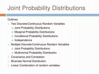
Probability: The Study of Randomness Random Variables. Chapters 4.3 and 4.4. Objectives (Chapters 4.3 and 4.4). Random variables Discrete random variables Continuous random variables Normal probability distributions Mean of a random variable Law of large numbers

E N D
Probability: The Study of RandomnessRandom Variables Chapters 4.3 and 4.4
Objectives (Chapters 4.3 and 4.4) Random variables • Discrete random variables • Continuous random variables • Normal probability distributions • Mean of a random variable • Law of large numbers • Variance of a random variable • Rules for means and variances
Discrete random variables A random variable is a variable whose value is a numerical outcome of a random phenomenon. A basketball player shoots three free throws. We define the random variable X as the number of baskets successfully made. A discrete random variableX has a finite number of possible values. A basketball player shoots three free throws. The number of baskets successfully made is a discrete random variable (X). X can only take the values 0, 1, 2, or 3.
H - HHH H M - HHM H H - HMH M M - HMM M … … The probability distribution of a random variable X lists the values and their probabilities: The probabilities pi must add up to 1. A basketball player shoots three free throws. The random variable X is thenumber of baskets successfully made. HMM HHM MHM HMH MMM MMH MHH HHH
The probability of any event is the sum of the probabilities pi of the values of X that make up the event. A basketball player shoots three free throws. The random variable X is thenumber of baskets successfully made. What is the probability that the player successfully makes at least two baskets (“at least two” means “two or more”)? HMM HHM MHM HMH MMM MMH MHH HHH P(X≥2) = P(X=2) + P(X=3) = 3/8 + 1/8 = 1/2 What is the probability that the player successfully makes fewer than three baskets? P(X<3) = P(X=0) + P(X=1) + P(X=2) = 1/8 + 3/8 + 3/8 = 7/8 or P(X<3) = 1 – P(X=3) = 1 – 1/8 = 7/8
Continuous random variables • A continuous random variableX takes all values in an interval. • Example: There is an infinity of numbers between 0 and 1 (e.g., 0.001, 0.4, 0.0063876). • How do we assign probabilities to events in an infinite sample space? • We use density curves and compute probabilities for intervals. • The probability of any event is the area under the density curve for the values of X that make up the event. This is a uniform density curve for the variable X. The probability that X falls between 0.3 and 0.7 is the area under the density curve for that interval: P(0.3 ≤ X ≤ 0.7) = (0.7 – 0.3)*1 = 0.4 X
Height = 1 X Intervals The probability of a single event is meaningless for a continuous random variable. Only intervals can have a non-zero probability, represented by the area under the density curve for that interval. The probability of a single event is zero: P(X=1) = (1 – 1)*1 = 0 The probability of an interval is the same whether boundary values are included or excluded: P(0 ≤ X ≤ 0.5) = (0.5 – 0)*1 = 0.5 P(0 < X < 0.5) = (0.5 – 0)*1 = 0.5 P(0 ≤ X < 0.5) = (0.5 – 0)*1 = 0.5 P(X < 0.5 or X > 0.8) = P(X < 0.5) + P(X > 0.8) = 1 – P(0.5 < X < 0.8) = 0.7
0.125 0.5 0.25 0.125 0 2 0.5 1 1.5 We generate two random numbers between 0 and 1 and take Y to be their sum. Y can take any value between 0 and 2. The density curve for Y is: Height = 1. We know this because the base = 2, and the area under the curve has to equal 1 by definition. The area of a triangle is ½ (base*height). Y 0 1 2 What is the probability that Y is < 1? What is the probability that Y < 0.5?
Continuous random variable and population distribution % individuals with X such that x1 < X < x2 The shaded area under a density curve shows the proportion, or %, of individuals in a population with values of X between x1 and x2. Because the probability of drawing one individual atrandom depends on the frequency of this type of individual in the population, the probability is also the shaded area under the curve.
Normal probability distributions The probability distribution of many random variables is a normal distribution. It shows what values the random variable can take and is used to assign probabilities to those values. Example: Probability distribution of women’s heights. Here, since we chose a woman randomly, her height, X, is a random variable. To calculate probabilities with the normal distribution, we will standardize the random variable (z score) and use Table A.
N(64.5, 2.5) N(0,1) => Standardized height (no units) Reminder: standardizing N(m,s) We standardize normal data by calculating z-scores so that any Normal curve N(m,s) can be transformed into the standard Normal curve N(0,1).
As before, we calculate the z-scores for 68 and 70. For x = 68", For x = 70", What is the probability, if we pick one woman at random, that her height will be some value X? For instance, between 68 and 70 inches P(68 < X < 70)? Because the woman is selected at random, X is a random variable. N(µ, s) = N(64.5, 2.5) 0.9192 0.9861 The area under the curve for the interval [68" to 70"] is 0.9861 − 0.9192 = 0.0669. Thus, the probability that a randomly chosen woman falls into this range is 6.69%. P(68 < X < 70) = 6.69%
s = 0.2 oz. Lowest2% x = 8 oz. m = ? Inverse problem: Your favorite chocolate bar is dark chocolate with whole hazelnuts. The weight on the wrapping indicates 8 oz. Whole hazelnuts vary in weight, so how can they guarantee you 8 oz. of your favorite treat? You are a bit skeptical... To avoid customer complaints and lawsuits, the manufacturer makes sure that 98% of all chocolate bars weigh 8 oz. or more. The manufacturing process is roughly normal and has a known variability = 0.2 oz. How should they calibrate the machines to produce bars with a mean m such that P(x < 8 oz.) = 2%?
s = 0.2 oz. Lowest2% x = 8 oz. m = ? How should they calibrate the machines to produce bars with a mean m such that P(x < 8 oz.) = 2%? Here we know the area under the density curve (2% = 0.02) and we know x (8 oz.). We want m. In table A we find that the z for a left area of 0.02 is roughly z = -2.05. Thus, your favorite chocolate bar weighs, on average, 8.41 oz. Excellent!!!
Mean of a random variable The mean x bar of a set of observations is their arithmetic average. The meanµof a random variable X is a weighted average of the possible values of X, reflecting the fact that all outcomes might not be equally likely. A basketball player shoots three free throws. The random variable X is thenumber of baskets successfully made (“H”). HMM HHM MHM HMH MMM MMH MHH HHH The mean of a random variable X is also called expected value of X.
Mean of a discrete random variable For a discrete random variable X withprobability distribution the mean µof X is found by multiplying each possible value of X by its probability, and then adding the products. A basketball player shoots three free throws. The random variable X is thenumber of baskets successfully made. The mean µ of X is µ = (0*1/8) + (1*3/8) + (2*3/8) + (3*1/8) = 12/8 = 3/2 = 1.5
Mean of a continuous random variable The probability distribution of continuous random variables is described by a density curve. The mean lies at the center of symmetric density curvessuch as the normal curves. Exact calculations for the mean of a distribution with a skewed density curve are more complex.
Law of large numbers As the number of randomly drawn observations (n) in a sample increases, the mean of the sample (x bar) gets closer and closer to the population mean m. This is the law of large numbers. It is valid for any population. Note: We often intuitively expect predictability over a few random observations, but it is wrong. The law of large numbers only applies to really large numbers.
Variance of a random variable The variance and the standard deviation are the measures of spread that accompany the choice of the mean to measure center. The variance σ2X of a random variable is a weighted average of the squared deviations (X − µX)2 of the variable X from its mean µX. Each outcome is weighted by its probability in order to take into account outcomes that are not equally likely. The larger the variance of X, the more scattered the values of X on average. The positive square root of the variance gives the standard deviation σ of X.
Variance of a discrete random variable For a discrete random variable Xwith probability distribution andmean µX, the variance σ2of X is found by multiplying each squared deviation of X by its probability and then adding all the products. A basketball player shoots three free throws. The random variable X is thenumber of baskets successfully made.µX = 1.5. The variance σ2 of X is σ2= 1/8*(0−1.5)2 + 3/8*(1−1.5)2 + 3/8*(2−1.5)2 + 1/8*(3−1.5)2 = 2*(1/8*9/4) + 2*(3/8*1/4) = 24/32 = 3/4 = .75
Rules for means and variances If X is a random variable and a and b are fixed numbers, then µa+bX= a + bµX σ2a+bX= b2σ2X If X and Y are two independent random variables, then µX+Y= µX+ µY σ2X+Y= σ2X+ σ2Y If X and Y are NOT independent but have correlation ρ, then µX+Y= µX+ µY σ2X+Y= σ2X+ σ2Y + 2ρσXσY
$$$ Investment You invest 20% of your funds in Treasury bills and 80% in an “index fund” that represents all U.S. common stocks. Your rate of return over time is proportional to that of the T-bills (X) and of the index fund (Y), such that R = 0.2X + 0.8Y. Based on annual returns between 1950 and 2003: • Annual return on T-bills µX = 5.0% σX = 2.9% • Annual return on stocks µY = 13.2% σY = 17.6% • Correlation between X and Yρ = −0.11 µR = 0.2µX + 0.8µY = (0.2*5) + (0.8*13.2) = 11.56% σ2R = σ20.2X + σ20.8Y + 2ρσ0.2Xσ0.8Y = 0.2*2σ2X + 0.8*2σ2Y + 2ρ*0.2*σX*0.8*σY = (0.2)2(2.9)2 + (0.8)2(17.6)2 + (2)(−0.11)(0.2*2.9)(0.8*17.6) = 196.786 σR = √196.786 = 14.03% The portfolio has a smaller mean return than an all-stock portfolio, but it is also less risky.
Probability: The Study of RandomnessGeneral Probability Rules Chapter 4.5
Objectives (Chapter 4.5) General probability rules • General addition rules • Conditional probability • General multiplication rules • Tree diagrams • Bayes’s rule
General addition rules General addition rule for any two events A and B: The probability that A occurs, B occurs, or both events occur is: P(A or B) = P(A) + P(B) – P(A and B) What is the probability of randomly drawing either an ace or a heart from a deck of 52 playing cards? There are 4 aces in the pack and 13 hearts. However, 1 card is both an ace and a heart. Thus: P(ace or heart) = P(ace) + P(heart) – P(ace and heart) = 4/52 + 13/52 - 1/52 = 16/52 ≈ .3
Conditional probability Conditional probabilities reflect how the probability of an event can change if we know that some other event has occurred/is occurring. • Example: The probability that a cloudy day will result in rain is different if you live in Los Angeles than if you live in Seattle. The conditional probability of event B given event A is:(provided that P(A) ≠ 0)
General multiplication rules • The probability that any two events, A and B, both occur is: P(A and B) = P(A)P(B|A) This is the general multiplication rule. • If A and B are independent, then P(A and B) = P(A)P(B) (A and B are independent when they have no influence on each other’s occurrence.) • What is the probability of randomly drawing either an ace or heart from a deck of 52 playing cards? There are 4 aces in the pack and 13 hearts. • P(heart|ace) = 1/4 P(ace) = 4/52 • P(ace and heart) = P(ace)* P(heart|ace) = (4/52)*(1/4) = 1/52 Notice that heart and ace are independent events.
Tree diagram for chat room habits for three adult age groups 0.47 Internet user Probability trees Conditional probabilities can get complex, and it is often a good strategy to build a probability tree that represents all possible outcomes graphically and assigns conditional probabilities to subsets of events. P(chatting) = 0.136 + 0.099 + 0.017 = 0.252 About 25% of all adult Internet users visit chat rooms.
Diagnosis sensitivity 0.8 Disease incidence Positive Cancer 0.0004 False negative Negative 0.2 Mammography 0.1 False positive Positive 0.9996 No cancer Negative Incidence of breast cancer among women ages 20–30 0.9 Diagnosis specificity Mammography performance Breast cancer screening If a woman in her 20s gets screened for breast cancer and receives a positive test result, what is the probability that she does have breast cancer? She could either have a positive test and have breast cancer or have a positive test but not have cancer (false positive).
Diagnosis sensitivity Disease incidence Positive Cancer False negative Negative Mammography False positive Positive No cancer Negative Diagnosis specificity 0.8 0.0004 0.2 0.1 0.9996 Incidence of breast cancer among women ages 20–30 0.9 Mammography performance Possible outcomes given the positive diagnosis: positive test and breast cancer or positive test but no cancer (false positive). This value is called the positive predictive value, or PV+. It is an important piece of information but, unfortunately, is rarely communicated to patients.
Bayes’s rule An important application of conditional probabilities is Bayes’s rule. It is the foundation of many modern statistical applications beyond the scope of this textbook. * If a sample space is decomposed in k disjoint events, A1, A2, … , Ak— none with a null probability but P(A1) + P(A2) + … + P(Ak) = 1, * And if C is any other event such that P(C) is not 0 or 1, then: However, it is often intuitively much easier to work out answers with a probability tree than with these lengthy formulas.
Diagnosis sensitivity Disease incidence Positive Cancer False negative Negative Mammography False positive Positive No cancer Negative Diagnosis specificity If a woman in her 20s gets screened for breast cancer and receives a positive test result, what is the probability that she does have breast cancer? 0.8 0.0004 0.2 0.1 0.9996 Incidence of breast cancer among women ages 20–30 0.9 Mammography performance This time, we use Bayes’s rule: A1 is cancer, A2 is no cancer, C is a positive test result.