Kinematics of the horizontal wind field

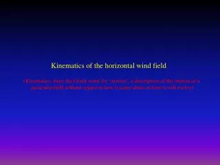
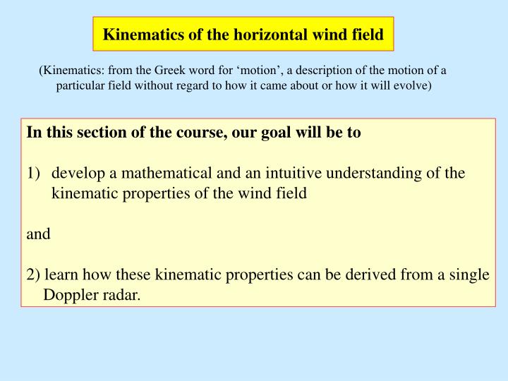
1. Kinematics of the horizontal wind field (Kinematics: from the Greek word for ‘motion’, a description of the motion of a particular field without regard to how it came about or how it will evolve) • In this section of the course, our goal will be to • develop a mathematical and an intuitive understanding of the • kinematic properties of the wind field • and • 2) learn how these kinematic properties can be derived from a single • Doppler radar.

2. Kinematics of the horizontal wind field (Kinematics: from the Greek word for ‘motion’, a description of the motion of a particular field without regard to how it came about or how it will evolve) y N V v To derive a mathematical expression for the key kinematic properties of the wind field we will use the coordinate system on the right. W E u x S y We will use a technique call Taylor Expansion to estimate the wind field at an arbitrary point x,y from the wind at a nearby point x0, y0 x, y x0, y0 x

3. A Taylor expansion is an infinite series of terms that use first, second, and higher order derivatives to determine a periodic function. For simplicity, lets assume that x0, y0 is the origin 0,0 and that we can obtain an adequate estimate of u,v by retaining only the first derivatives. We are assuming that over the small distance the u and v field vary linearly. Then…

4. Let’s take a simple step and write each derivative term as (for example) :

5. From before: (1) (2) Now we will write two nonsense equations (3) (4) Now we add (1) and (3). We also separately add (2) and (4). Then we rearrange the terms and get…………

6. Translation Divergence Shearing Deformation Relative Vorticity Stretching Deformation Any wind field that varies linearly can be characterized by these five distinct properties. Non-linear wind fields can be closely characterized by these properties.

7. y x Translation The effect of translation on a fluid element: Change in location, no change in area, orientation, shape

8. y Divergence (d > 0) Convergence (d < 0) The effect of convergence on a fluid element: x Change in area, no change in orientation, shape, location

9. y Positive (cyclonic) vorticity ( > 0). Negative (anticyclonic) vorticity ( < 0) The effect of negative vorticity on a fluid element: x Change in orientation, no change in area, shape, location

10. y E-W Stretching Deformation (D1 > 0). N-S Stretching Deformation (D1 < 0). The effect of stretching deformation on a fluid element: x Change in shape, no change in area, orientation, location Axis of dilitation Axis of contraction

11. y SW-NE Shearing Deformation (D1 > 0). NW-SE Shearing Deformation (D1 < 0). The effect of shearing deformation on a fluid element: x Change in shape, no change in area, orientation, location

12. VELOCITY-AZIMUTH DISPLAY (VAD) PROCESSING OF RADIAL VELOCITY DATA FROM A DOPPLER RADAR A technique for the measurement of kinematic properties of a wind field in widespread echo coverage using a single Doppler radar

13. RADAR GEOMETRY

14. Equation for radial velocity in terms of wind components: (1) Where a = elevation angle, b = azimuth angle Vr = radial velocity Vx = east-west wind component Vy = north-south wind component, Vf =up-down total particle motion (air motion +particle terminal velocity) We will assume that the velocity gradient across a ring varies linearly so that: (2) (3)

15. Let us now put (2) and (3) into (1) Also use the identities: to get… note

16. Write previous equation as a Fourier series where and the coefficients are:

17. The Fourier components are related to the kinematic properties of the wind East-west component of wind North-South component of wind Up-down component of wind+fall velocity Divergence Stretching deformation Shearing deformation

18. Contains information about Divergence and total fall velocity of the particles Contains information about the horizontal wind speed and direction Contains information about the flow deformation and its orientation

19. Kinematic properties of the wind can be obtained from the Fourier Coefficients Divergence Wind velocity for b1 negative Wind direction for b1 positive

20. Deformation for b2 negative Axis of dilatation for b2 positive

21. Data taken along a ring in a VAD scan at range 5922 m and altitude 2582 m at elevation angle 17.7° in a winter storm Derived Fourier Spectral Components Data points are radial velocities Radial velocity Line is best fit line Azimuth angle Azimuth angle

22. Data taken along a ring in a VAD scan at range 2825 m and altitude 253 m at elevation angle 0.5° in a winter storm Not all radial velocity data is so well behaved – these “bad data” points must be removed before regression to find coefficients

23. Analysis of data on individual rings to determine kinematic properties 1. Dealiasing (unfolding) velocities Step up one ring at a time – if fold occurs, unfold the velocities Measure wind at ground to determine initial folding factor 2. Remove unrepresentative data Ground clutter (bias toward zero velocity) Low echo power (noisy velocity) Low reflectivity factor (noisy velocity)

24. 3. Remove data unrepresentative of large scale motions as well as “bad” data • Do regression • Any point that deviates from regression line by • DV > M m/s or by more then n standard deviations is removed • Do regression again • Repeat b • Do final regression

25. Goal of VAD processing: Determine the Fourier coefficients, ai, from the radial velocity data on rings Mathematical technique: Least squares regression method (use matrix algebra) Define: where i = 1,2,…5 And N = number of samples on ring Column vector Then………… Matrix

26. Where:

27. 4. Calculate Fourier Coefficients using Least Squares

28. 4. Calculate Vertical profiles of radar reflectivity wind speed, wind direction, deformation, axis of dilitation. Number of data points on rings on a cone and standard deviation of fit on each ring Radar reflectivity factor profile

29. 4. Calculate Vertical profiles of wind speed, wind direction, deformation, axis of dilitation, radar reflectivity. Wind speed and wind direction Deformation and axis of dilitation

30. Extended Velocity Azimuth Display Goal: To separate the horizontal divergence from the hydrometeor fall velocity in the zeroth harmonic Let’s rewrite equation: Equation of a straight line

31. EVAD analysis is done in layers. Each ring gives one data point that is used in a least squares regression to obtain D and Vf within the layer At high elevation angles, Vf contributes most to zeroth harmonic At low elevation angles, D contributes most to zeroth harmonic

32. Net effect: Average divergence and particle total fall velocity are obtained in each layer Note: There are a number of mathematical complexities associated with EVAD that I am glossing over. If you are interested in using EVAD techniques, you should consult Matejka, Thomas, Srivastava, Ramesh C. 1991: An Improved Version of the Extended Velocity-Azimuth Display Analysis of Single-Doppler Radar Data. Journal of Atmospheric and Oceanic Technology: Vol. 8, No. 4, pp. 453–466.

33. Calculation of vertical motion Once the divergence has been obtained in layers, the continuity equation (which describes the conservation of mass), can be used to calculate the vertical motion within the VAD analysis region. Where: The continuity equation can be integrated upward, downward, or both (with appropriate weighting – we will discuss this in the section of the course on dual-Doppler analysis)

34. Equations for upward and downward integration for w Once w is calculated, the particles terminal velocity can be determined from:

35. Examples of EVAD analyses from a major ice storm in Champaign, IL From: Rauber, Robert M., Ramamurthy, Mohan K., Tokay, Ali. 1994: Synoptic and Mesoscale Structure of a Severe Freezing Rain Event: The St. Valentine's Day Ice Storm.Weather and Forecasting: Vol. 9, No. 2, pp. 183–208

36. Operational VAD calculation of winds from NEXRAD in Hurricane Jeanne (2004) From Jacksonville, FL radar VAD winds available from COD http://weather.cod.edu/analysis/analysis.radar.html