Download
1 / 25
250 likes | 488 Views
Lidar Meeting 2007. The Scatterometer is no longer a competitor for lidar winds. R. A. Brown 2007 Lidar Miami. The Scatterometer. RIP ( USA ). R. A. Brown 2007 Lidar Miami. UW; Patoux, ‘03. R. A. Brown 2007 Lidar Miami. Scatterometers in Space. SeaSat 1978.

E N D
Lidar Meeting 2007 The Scatterometer is no longer a competitor for lidar winds R. A. Brown 2007 Lidar Miami
The Scatterometer RIP (USA) R. A. Brown 2007 Lidar Miami
UW; Patoux, ‘03 R. A. Brown 2007 Lidar Miami
Scatterometers in Space SeaSat 1978 ERS -1 1991-95 ERS-2 1995-2001 ERS-2 1995-2001; 2003 - NSCAT 1996-97 QuickScat 1999 - SeaWinds1 1998-1998 SeaWinds2 2002 - 2002 ASCAT 2007 R. A. Brown 2007 Lidar Miami
Products R. A. Brown 2003 U. ConcepciÓn
Surface Pressures from Space R. A. Brown 2004 EGU
The solution for the PBL boundary layer (Brown, 1974, Brown and Liu, 1982), may be written U/VG = ei - e –z[e-iz + ieiz]sin +U2 where VG is the geostrophic wind vector, the angle between U10 and VG is [u*, HT, (Ta – Ts,)PBL] and the effect of the organized large eddies (OLE) in the PBL is represented by U2(u*, Ta – Ts, HT) This may be written: U/VG ={(u*), U2(u*), u*, zo(u*), VT(HT), (Ta – Ts), } Or U/VG = [u*, VT(HT), (Ta – Ts), , k, a] = {u*, HT, Ta – Ts}, for = 0.15, k= 0.4 and a = 1 In particular, VG = (u*,HT, Ta – Ts) n(P, , f) Hence P = n [u*(k, a, ), HT, Ta – Ts, , f ] fn(o) R. A. Brown 2006 AMS
SLP from Surface Winds • UW PBL similarity model joins two layers: • Use “inverse” PBL model to estimate from satellite . Get non-divergent field UGN. • Use Least-Square optimization to find best fit SLP to swaths • There is extensive verification from ERS-1/2, NSCAT, QuikSCAT UG (UGN ) R. A. Brown 2006 AMS
Dashed: ECMWF J. Patoux & R. A. Brown
Surface Pressures QuikScat analysis ECMWF analysis J. Patoux & R. A. Brown
UW + gradient wind EC ----- UW ___ The low is deeper, and the pressure gradients are stronger, especially where the winds are strong and where the streamlines are curved the most. This can be appreciated on the western flank of the low. The whole structure of the pressure field is affected by the gradient wind correction: it is more asymmetric, as well as deeper. Note that the uncorrected low is shallower than indicated by ECMWF, but that the corrected low is deeper than indicated by ECMWF. R. A. Brown 2003 U. ConcepciÓn
(JPL) JPL Project Local GCM nudge smoothed = Dirth (with ECMWF fields) UW Pressure field smoothed Raw scatterometer winds R. A. Brown 2006 AMS
The nonlinear solution applied to satellite surface winds yields accurate surface pressure fields. These data show: * Agreement between satellite and ECMWF pressure fields indicate that both Scatterometer winds and the nonlinear PBL model (VG/U10) are accurate within 2 m/s. * A 3-month, zonally averaged offset angle <VG, U10> of 19° suggests the mean PBL state is near neutral (the angle predicted by the nonlinear PBL model). * Swath deviation angle observations infer thermal wind and stratification. * Higher winds are obtained from pressure gradients and used as surface truth (rather than from GCM or buoy winds). * VG (pressure gradients) rather than U10 is being used to initialize GCMs R. A. Brown 2006 AMS
The nonlinear solution applied to satellite surface winds yields accurate surface pressure fields. These data show: * Agreement between satellite and ECMWF pressure fields. This indicates that both the Scatterometer winds and the nonlinear PBL model (VG/U10) are accurate within 2 m/s. * A 3-month, zonally averaged offset angle <VG, U10> of 19° suggests the mean PBL state is near neutral (the angle predicted by the nonlinear PBL model). * Swath deviation angle observations can be used to infer thermal wind and stratification. * Higher winds are obtained from pressure gradients and used as surface truth (rather than from GCM or buoy winds). * VG (pressure gradients) rather than U10 could be used to initialize GCMs R. A. Brown 2006 AMS
NCEP real time forecasts use PBL model Even the best NCEP analysis, used as the first guess in the real time forecasts, is improved with the QuikScat surface pressure analyses. R. A. Brown 2007 Lidar Miami
This is the 0600 UTC Ocean Prediction Center hand drawn surface analysis superimposed over the GOES12 0615UTC Image.
L 999 L 993 L 1003 This is a cut and paste of two QuikScat passes.
This is a composite of two runs of the model using the 0549 QuikSCAT pass and the 0648 QuikSCAT pass.
This is the composite of three consecutive runs of the uwpbl model using the 0543, 0648 and 0834 QuikSCAT passes superimposed on the GOES 12 image from 0645 UTC
This is the Ocean Prediction Center hand drawn surface analysis 0526 0600 UTC with the surface vorticity field from the uwpbl model overlaid. The vorticity field is a composite of three passes (0543, 0648 and 0834 UTC); it shows the locations of the frontal zones well.
a b 991 999 GFS Sfc Analysis 10 Jan 2005 0600 UTC QuikSCAT 10 Jan 2005 0709 UTC c d 984 996 982 996 OPC Sfc Analysis and IR Satellite Image 10 Jan 2005 0600 UTC UWPBL 10 Jan 2005 0600 UTC This example is from 10 January 2005 0600UTC. Numerical guidance from the 0600UTC GFS model run (a) indicated a 999 hPa low at 43N, 162E. QuikScat winds (b) suggested strong lows --- OPC analysis uses 996. UW-PBL analysis indicates 982.
Programs and Fields available onhttp://pbl.atmos.washington.eduQuestionsto rabrown, Ralph orjerome @atmos.washington.edu • Direct PBL model: PBL_LIB. (’75 -’05) An analytic solution for the PBL flow with rolls, U(z) = f( P, To , Ta , ) • The Inverse PBL model: Takes U10 field and calculates surface pressure field P (U10 , To , Ta , ) (1986 - 2005) • Pressure fields directly from the PMF: P (o) along all swaths (exclude 0 - 5° lat.?) (2001) (dropped in favor of I-PBL) • Global swath pressure fields for QuikScat swaths (with global I-PBL model) (2005) • Surface stress fields from PBL_LIB corrected for stratification effects along all swaths (2006) R. A. Brown 2007 Lidar Miami
R. A. Brown 2005 EGU R. A. Brown, J. Patoux
In this case, the system is decaying but a secondary low is developing behind the remnants of the cold front. Note also the correspondance between convergence and clouds. R. A. Brown 2003 U. ConcepciÓn