Download

1 / 22
220 likes | 410 Views
EE 212 Passive AC Circuits. Lecture Notes 2b. Application of Thevenin’s Theorem Thevenin's Theorem is specially useful in analyzing power systems and other circuits where one particular segment in the circuit (the load) is subject to change. Source Impedance at a Power System Bus

E N D
EE 212 Passive AC Circuits Lecture Notes 2b EE 212
Application of Thevenin’s Theorem Thevenin's Theorem is specially useful in analyzing power systems and other circuits where one particular segment in the circuit (the load) is subject to change. Source Impedance at a Power System Bus The source impedance value (or the network impedance at the power system bus) can be obtained from the utility for all the sub-stations of a power grid. This is the Thevenin Impedance seen upstream from the sub-station bus. The Thevenin Voltage can be measured at the bus (usually the nominal or rated voltage at the bus). Thevenin equivalent at the sub-station is important to determine cable, switchgear and equipment ratings, fault levels, and load characteristics at different times. EE 212
A A Linear Circuit Z I B B Norton’s Theorem Any linear two terminal network with sources can be replaced by an equivalent current source in parallel with an equivalent impedance. Current source I is the current which would flow between the terminals if they were short circuited. Equivalent impedance Z is the impedance at the terminals (looking into the circuit) with all the sources reduced to zero. EE 212
Z A A Z ~ E I B B Thevenin Equivalent E = IZ Norton Equivalent I = E / Z Note: equivalence is at the terminals with respect to the external circuit. EE 212
Superposition Theorem If a linear circuit has 2 or more sources acting jointly, we can consider each source acting separately (independently) and then superimpose the 2 or more resulting effects. • Steps: • Analyze the circuit considering each source separately • To remove sources, short circuit V sources and open circuit I sources • For each source, calculate the voltages and currents in the circuit • Sum the voltages and currents Superposition Theorem is very useful when analyzing a circuit that has 2 or more sources with different frequencies. EE 212
an = bn = Non-sinusoidal Periodic Waveforms A non-sinusoidal periodic waveform, f(t) can be expressed as a sum of sinusoidal waveforms. This is known as a Fourier series. Fourier series is expressed as: f(t) = a0 + (an Cos nwt) + (bn Sin nwt) where, a0 = average over one period (dc component) = for n > 0 EE 212
bn= = an = = 0 f(t) = a0 + (ancos nωt) + (bnsin nωt) = (sin ωt + sin 3ωt + sin 5ωt + …..) Non-sinusoidal Periodic Waveforms: Square Waveform f(t) = 1 for 0 ≤ t ≤ T/2 = -1 for T/2 ≤ t ≤ T a0 = average over one period = 0 EE 212 http://homepages.gac.edu/~huber/fourier/index.html
Linear AC Circuits with Non-Sinusoidal Waveforms A linear circuit with non-sinusoidal periodic sources can be analyzed using the Superposition Theorem. • Express the non-sinusoidal function by its Fourier series. • That is, the periodic source will be represented as multiple sinusoidal sources of different frequencies. Use Superposition Theorem to calculate voltages and currents for each element in the series. Calculate the final voltages and currents by summing up all the harmonics. EE 212
Vrms = √(v0 2 + v1 2 + v2 2 + v3 2 + …) peak values • Irms = √( i0 2 + i1 2 + i2 2 + i3 2 + …) peak values • Vrms = √V02 + V1rms2 + V2rms2 + V3rms2 + … P = V0 I0 + v1 i1 cos1 + v2 i2 cos2 + .. v1 i1 sin 1 + v2 i2 sin 2 + .. Q = Equations for RMS Values (V, I) and Power P = |Irms| 2 R EE 212
5W + 0.02 H v(t) - Example: Non-sinusoidal AC source Find the RMS current and power supplied to the circuit elements. The circuit is energized by a non-sinusoidal voltage v(t), where: v(t) = 100 + 50 sin wt + 25 sin 3wt volts, and w = 500 rad/s EE 212
i v ~ Linear Circuit with AC Excitation Input signal, v = Vm sin wt Response to a sinusoidal input is also sinusoidal. Has the same frequency, but may have different phase angle. Response i = Im sin (wt + ) where is the phase angle between v and i Power Factor: cosine of the angle between the current and voltage, i.e. p.f. = cos If is + ve, i leads v leading p.f. If is - ve, i lags v lagging p.f. EE 212
I V Across Resistor – Unity p.f. Voltage and Current are in phase v(t) = Vm sin wt i(t) = Im sin wt i.e., angle between v and i, = 00 p.f. = cos = cos 00 = 1 Phasor Diagram EE 212
V I Clock-wise lagging Across Inductor – Lagging p.f. Current lags Voltage by 900 v(t) = Vm sin wt i(t) = Im sin (wt-900) angle between v and i, = 900 p.f. = cos = cos 900 = 0 lagging Phasor Diagram EE 212
I V Across Capacitor – Leading p.f. Current leads Voltage by 900 v(t) = Vm sin wt i(t) = Im sin (wt+900) angle between v and i, = 900 p.f. = cos = cos 900 = 0 leading Phasor Diagram EE 212
i v p(t) = cos θ – cos(2ωt-θ) p(t) = cosθ(1-cos2ωt) + sinθ·sin2ωt Power v = Vm sin ωt volts i = Im sin(ωt - θ) A Instantaneous Power, p(t) = v(t) · i(t) p(t) = Vm sin ωt · Im sin(ωt - θ) Real Power, P = average value of p(t) = Vrms·Irms·cos θ Reactive Power, Q = peak value of power exchanged every half cycle = Vrms·Irms·sin θ EE 212
Real and Reactive Power Reactive Power, Q Real (Active) Power, P • useful power • measured in watts • capable of doing useful work, e.g. , lighting, heating, and rotating objects • hidden power • measured in VAr • related to power quality Sign Convention: Power used or consumed: + ve Power generated: - ve EE 212
Real and Reactive Power (continued) • Source – AC generator: P is – ve • Induction gen: Q is +ve Synchronous: Q is + or –ve • Load – component that consumes real power, P is + ve • Resistive: e.g. heater, light bulbs, p.f.=1, Q = 0 • Inductive: e.g. motor, welder, lagging p.f., Q = + ve • Capacitive: e.g. capacitor, synchronous motor (condensor), leading p.f., Q = - ve • Total Power in a Circuit is Zero EE 212
p.f. = Im jQ |S| Q Re P Complex Power Complex Power, S = V I* (conjugate of I) S = P + jQ in Rectangular Form P - Real Power Q – Reactive Power S = |S| / in Polar Form - Power Factor Angle |S| - Apparent Power measured in VA P = |S| cos = |V| |I| cos Q = |S| sin = |V| |I| sin P = |I|2 R Q = |I|2 X |S| = |V|·|I| Power ratings of generators & transformers in VA, kVA, MVA EE 212
Motor 5 hp, 0.8 p.f. lagging 100% efficiency Welder 4+j3 W Heater 5 kW 120 volts @60 Hz Examples: Power 1: V = 10/100V, I = 20/50A. Find P, Q 2: What is the power supplied to the combined load? What is the load power factor? EE 212
Power Factor Correction Most loads are inductive in nature, and therefore, have lagging p.f. (i.e. current lagging behind voltage) Typical p.f. values: induction motor (0.7 – 0.9), welders (0.35 – 0.8), fluorescent lights (magnetic ballast 0.7 – 0.8, electronic 0.9 - 0.95), etc. Capacitance can be added to make the current more leading. EE 212
Power Factor Correction(continued) • P.F. Correction usually involves adding capacitor (in parallel) to the load circuit, to maximize the p.f. and bring it close to 1. • The load draws less current from the source, when p.f. is corrected. • Benefits: • - • Therefore, p.f. is a measure of how efficiently the power supply is being utilized EE 212
Motor 5 hp, 0.8 p.f. lagging 100% efficiency Welder 4+j3 W Heater 5 kW 120 volts @60Hz Example: P.F. Correction What capacitor is required in parallel for p.f. correction? Find the total current drawn before and after p.f. correction. EE 212