Download
1 / 40
400 likes | 488 Views
Approximate genealogical inference. Gil McVean Department of Statistics, Oxford. Motivation. We have a genome’s worth of data on genetic variation We would like to use these data to make inferences about multiple processes: recombination, mutation, natural selection, demographic history.

E N D
Approximate genealogical inference Gil McVean Department of Statistics, Oxford
Motivation • We have a genome’s worth of data on genetic variation • We would like to use these data to make inferences about multiple processes: recombination, mutation, natural selection, demographic history
Example I: Recombination • In humans, the recombination rate varies along a chromosome • Recombination has characteristic influences on patterns of genetic variation • We would like to estimate the profile of recombination from the variation data – and learn about the factors influencing rate
Example II: Genealogical inference • The genealogical relationships between sequences are highly informative about underlying processes • We would like to estimate these relationships from DNA sequences • We could use these to learn about history, selection and the location of disease-associated mutations
Modelling genetic variation • We have a probabilistic model that can describe the effects of diverse processes on genetic variation: The coalescent • Coalescent modelling describes the distribution of genealogical relationships between sequences sampled from idealised populations • Patterns of genetic variation result from mapping mutations on the genealogy
Where do these trees come from? Present day
Ancestry of current population Present day
Ancestry of sample Present day
The coalescent: a model of genealogies Most recent common ancestor (MRCA) coalescence Ancestral lineages Present day time
Coalescent modelling describes the distribution of genealogies
Generalising the coalescent • The impact of many different forces can readily be incorporated into coalescent modelling • With recombination, the history of the sample is described by a complex graph in which local genealogical trees are embedded – called the ancestral recombination graph or ARG Ancestral chromosome recombines
Coalescent-based inference • We would like to use the coalescent model to drive inference about underlying processes • Generally, we would like to calculate the likelihood function • However, there is a many-to-one mapping of ARGs (and genealogies) to data • Consequently, we have to integrate out the ‘missing-data’ of the ARG • This can only be done using Monte Carlo methods (except in trivial examples)
tMRCA Coalescence Mutation t7 t6 Coalescence t5 Coalescence t4 Mutation t3 Coalescence t2 Recombination t1 Coalescence t = 0 time time time time time time time
A problem and a possible solution • Efficient exploration of the space of ARGs is a difficult problem • The difficulties of performing efficient exact genealogical inference (at least within a coalescent framework) currently seem insurmountable • There are several possible solutions • Dimension-reduction • Approximate the model • Approximate the likelihood function • One approach that has proved useful is to combine information from subsets of data for which the likelihood function can be estimated • Composite likelihood
Example I: Recombination rate estimation • We can estimate the likelihood function for the recombination fraction separating two SNPs • To approximate the likelihood for the whole data set, we simply multiply the marginal likelihoods (Hudson 2001) • The method performs well in point-estimation
DlnL DlnL R R Full likelihood Composite-likelihood approximation DlnL R 15 7 1 1 2 7 2 2 4 2 3 1 1 1 1
Good and bad things about CL • Good things • Estimation using CL can be made very efficient • It performs well in simulations • It can generalise to variable recombination rates • Bad things • It throws away information • It is NOT a true likelihood • It typically underestimates uncertainty because of ‘double-counting’
Split blocks Merge blocks Change block size Change block rate Fitting a variable recombination rate • Use a reversible-jump MCMC approach (Green 1995) SNP positions Cold Hot
Acceptance rates • Include a prior on the number of change points that encourages smoothing Hastings ratio Composite likelihood ratio Ratio of priors Jacobian of partial derivatives relating changes in parameters to sampled random numbers
rjMCMC in action • 200kb of the HLA region – strong evidence of LD breakdown
How do you validate the method? • Concordance with rate estimates from sperm-typing experiments at fine scale • Concordance with pedigree-based genetic maps at broad scales
Rates estimated from sperm Jeffreys et al (2001) Strong concordance between fine-scale rate estimates from sperm and genetic variation Rates estimated from genetic variation McVean et al (2004)
We have generated a map of hotspots across the human genome Myers et al (2005)
We have identified DNA sequence motifs that explain 40% of all hotspots Myers et al (2008)
Age of mutation Date of population founding Migration and admixture Example II: Estimating local genealogies ?
Two sequence case • Any pair of haplotypes will have regions of high and low divergence • We can combine HMM structures with numerical techniques (Gaussian quadrature) to estimate the marginal likelihood surface at a given position, x • We can further approximate the likelihood surface by fitting a scaled gamma distribution • This massively reduces the computational load of subsequent steps • In the case of no recombination the truth is a scaled gamma distribution 010111000000000000000000000000000111001110000 001001010000000000000000000000000101000100010
t Pr( ) 0 } a b Combining surfaces • Suppose we have a partially-reconstructed tree • We can approximate the probability of any further step in the tree using the composite-likelihood (assumes un-coalesced ancestors are independent draws from stationary distribution)
An important detail • Actually, don’t use exactly this construction • Use a ‘nearest-neighbour’ construction • Each lineage chooses a nearest neighbour • Choose which nearest-neighbour event to occur • Choose a time for the nearest-neighbour event • Still uses composite likelihood
Building the tree • We can use these functions to choose (e.g. maximise or sample) the next event • The gamma approximation leads to an efficient algorithm for estimating the local genealogy that has the same time and memory complexity of neighbour-joining • This mean it can be applied to large data sets
Desirable properties of the algorithm • It can be fully stochastic (unlike NJ, UPGMA, ML) • It returns the prior in the absence of data: • It returns the truth in the limit of infinite data: • It is correct for a single SNP: • It is close to the optimal proposal distribution (as defined by Stephens and Donnelly 2000) in the case of no recombination • It uses much of the available information • It is fast – time complexity in n the same as for NJ
Example: mutation rate = recombination rate Simulations The true tree at 0.5 q = 10, R = 10
How to evaluate tree accuracy? • Specific applications will require different aspects of the estimated trees to be more or less accurate • Nevertheless, a general approach is to compare the representation of bi-partitions in the true tree to estimated ones • Rather than require 100% accuracy in predicting a bi-partition, we can (for every observed bi-partition) find the ‘most similar’ bi-partition in the estimated tree • We should also weight by the branch length associated with each bi-partition
Simple distance weighting (UPGMA) Single sample from posterior Average weighted max r2 = 0.59 Average weighted max r2 = 0.96 n = 100, q = 20, R = 30 (hotspots)
Open questions • Obtaining useful estimates of uncertainty • Power transformations of composite likelihood function • Using larger subsets of the data • E.g. quartets
Acknowledgements • Many thanks to • Oxford statistics • Simon Myers, Chris Hallsworth, Adam Auton, Colin Freeman, Peter Donnelly • Lancaster • Paul Fearnhead • International HapMap Project