Download
1 / 38
380 likes | 525 Views
Approximate Inference Using Planar Graph Decomposition. Amir Globerson and Tommi Jaakkola In Advances in Neural Information Processing Systems 19 , 2006. Presented by Jonathan Huang at SELECT Lab, 12/12/06. The Ising Model. Let G=(V,E) be a graph

E N D
Approximate Inference Using Planar Graph Decomposition Amir Globerson and Tommi Jaakkola In Advances in Neural Information Processing Systems 19, 2006 Presented by Jonathan Huang at SELECT Lab, 12/12/06
The Ising Model • Let G=(V,E) be a graph • The Ising Model of statistical physics is a distribution on binary variables x1,x2,…,xN which takes the form: • xi {-1,+1} • Z() is the partition function which normalizes the distribution. Field Strengths Coupling Strengths
The Ising Model • For example, if G=(V,E) is the following graph: • Then: x1 x2 x3 x4
Zero External Field • If there are only interaction potentials, we will say that there is no external field: • (i=0)
The Ising Model • In general, the partition function Z() is intractable to compute because it involves summing over all joint settings of x1,x2,…,xN • This paper presents a way to approximately compute the partition function
Outline • Some Graph Theory Definitions • Exact Solution for Planar Ising models with zero external field • Partition Function bounds via the Planar Decomposition • Bound Optimization • Compare to Tree Reweighting approximations
Planar Graphs • A planar graph is a graph which can be drawn on a plane such that no edges intersect Planar Non-Planar
The Dual Graph • Given a planar graph G, there exists a dual graph G* which has a vertex for each face of G and an edge for each edge in G joining two neighboring faces G (G* shown in red)
Plane Triangulations • A plane triangulation of a planar graph G is obtained by adding edges until all the faces of the resulting graph are bounded by triangles
Plane Triangulation Dual • The vertices of the dual of a plane triangulated graph are all of degree 3:
Perfect Matchings • A perfect matching is a subset of edges F E such that every vertex in G has exactly one edge in F incident on it • If the edges are weighted, then the weight of the matching is defined to be the product of the weights of the edges in the matching
Outline • Some Graph Theory Definitions • Exact Solution for Planar Ising models with zero external field • Partition Function bounds via the Planar Decomposition • Bound Optimization • Compare to Tree Reweighting approximations
Exact Calculation of the Partition Function • Let G be the planar graph associated with the given Ising model • We assume zero external field • Strategy: • Convert G to a new weighted graph GPM for which Z() is equal to the sum over all perfect matchings • Sum over all perfect matchings
Agreement Edge Sets • A set of edges E* in a triangulated graph G is an agreement edge set (AES) if for every triangle face F in G, either: • The edges in F are all in E* • Or, exactly one of the edges in F is in E or
Agreement Edge Sets (cont.) • There is a correspondence between pairs of assignments (x,-x) and Agreement Edge Sets • Map an assignment x to the set of edges such that xi=xj
Agreement Edge Sets (cont.) • The contribution of a given assignment x is: • If x corresponds to the AES E*, then its contribution can be written as: • (the point of all this is that a sum over all assignments is equivalent to a sum over all AESs)
Converting G to GPm • Step 0: Start with a Planar Graph G
Converting G to GPm • Step 1: Triangulate G to get GTri • Set new edge weights to be 1 • This defines a new Ising model with the same normalization • We’d like to sum over the Agreement Edge Sets of GTri because:
Converting G to GPm • Step 2: Dualize GTri and replace each vertex with three vertices that are connected to each other and each of the three is connected to one of the neighbors of the original vertex • Call this new graph GPM
The Correspondence • Claim: Every Perfect Matching in GPM corresponds to an agreement edge set in GTri • This shows that a sum over agreement edge sets is equivalent to a sum over perfect matchings
The Correspondence (cont.) • (An illustration): A triangle from GTri Its dual vertex and edges in GPM
Exact Calculation of the Partition Function • Let G be the planar graph associated with the given Ising model • We assume zero external field • Strategy: • Convert G to a new weighted graph GPM for which Z() is equal to the sum over all perfect matchings • Sum over all perfect matchings
Summing over all Perfect Matchings • This is #P-complete for general graphs • If all the weights are 1, this is the matrix permanent problem • But for planar graphs (like GPM), it can be computed in poly-time using Pfaffians
What are Pfaffians?? • Let A be a skew-symmetric matrix • Theorem: The determinant of A can be written as the square of a polynomial in the matrix entries of A • Due to Sir Arthur Cayley (not Pfaff) • Define the Pfaffian of A to be:
Pfaffians and Perfect Matchings • Let H be a planar graph with weights wij • Direct the edges of H such that for each face, the number of clockwise-oriented edges on its perimeter is odd (this is called a Pfaffian Orientation) • Define a skew-symmetric matrix P(H): 1 1 1 1 1 1 1 1 1 1 1 1
Pfaffians and Perfect Matchings • Theorem: Pf(P(H)) is the sum over all weighted matchings on H • The partition function of a planar binary graph with pure interaction potentials can be computed in polynomial time!
Outline • Some Graph Theory Definitions • Exact Solution for Planar Ising models with zero external field • Partition Function bounds via the Planar Decomposition • Bound Optimization • Compare to Tree Reweighting approximations
Partition Function bounds via the Planar Decomposition • Now consider a non-planar G over binary variables with zero external field • Let G(r) be a set of spanning planar subgraphs of G • Let (r) be a set of potentials on the edges of G(r) • Extend (r) to be a set of potentials on the edges of G by setting potentials to be zero on edges not in G(r) • Z((r)) is the partition function on G(r) with respect to the parameters (r)
Partition Function bounds via the Planar Decomposition • Now given any distribution (r) on the Gr, • If: • Then by convexity of the log-partition function:
Outline • Some Graph Theory Definitions • Exact Solution for Planar Ising models with zero external field • Partition Function bounds via the Planar Decomposition • Bound Optimization • Compare to Tree Reweighting approximations
Bound Optimization • The goal is to make this bound as tight as possible:
Bound Optimization • Since the objective function is convex, the optimization is guaranteed to converge to globally optimal mixture coefficients and parameters for each spanning planar subgraph
Marginal Optimality Criterion • Let G(r), G(s) be two planar subgraphs that both contain the edge (i,j). • At the optimal parameter vector, they must agree on the marginal of (i,j) • So getting at marginal edge probabilities is easy: • Just use marginals from one of the planar subgraphs
Outline • Some Graph Theory Definitions • Exact Solution for Planar Ising models with zero external field • Partition Function bounds via the Planar Decomposition • Bound Optimization • Compare to Tree Reweighting approximations
External Fields • Suppose G is planar, but now consider a nonzero external field • Can rewrite the model in terms of pure interaction potentials by adding an additional node connected to all original variables • This break planarity =/ (extra edges not drawn here)
Experimental Evaluation • Compared performance of planar decomposition to tree reweighting on a 7x7 square lattice Red = Tree Reweighting results, Blue = Planar Decomposition Results
Conclusions • Pros • Better partition functions bounds than Tree Reweighted BP in many cases (except for singleton marginals) • Cons • Only defined for binary MRFs • The optimization is carried out explicitly over a set of planar subgraphs here, but in TRW, the optimization is implicitly over an exponential number of spanning trees • Also, the paper doesn’t compare to other approximate inference algorithms

![Beyond Trees: MRF Inference via Outer-Planar Decomposition [(To appear) CVPR ‘10]](https://cdn1.slideserve.com/1617336/beyond-trees-mrf-inference-via-outer-planar-decomposition-to-appear-cvpr-10-dt.jpg)