Download
1 / 36
430 likes | 540 Views
k. K ( q ). P. q. Wave front. P. S. a. R 2. R 1. March 22, 25 Fresnel zones. 10.3 Fresnel diffraction 10.3.1 Free propagation of a spherical wave Fresnel diffraction : For any R 1 and R 2 . Fraunhofer diffraction is a special case of Fresnel diffraction.

E N D
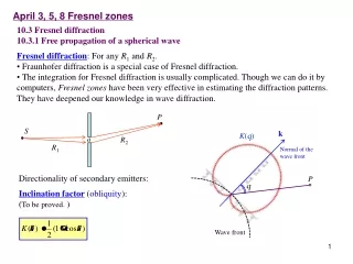
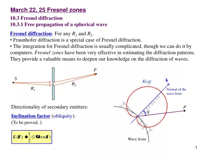
k K(q) P q Wave front P S a R2 R1 March 22, 25 Fresnel zones • 10.3 Fresnel diffraction • 10.3.1 Free propagation of a spherical wave • Fresnel diffraction: For any R1and R2. • Fraunhofer diffraction is a special case of Fresnel diffraction. • The integration for Fresnel diffraction is usually complicated, though we can do it by computers. Fresnel zones have been very effective in estimating the diffraction patterns. They provide a valuable means to deepen our knowledge on the diffraction of waves. Normal of the wave front Directionality of secondary emitters: Inclination factor(obliquity): (To be proved. )
Free propagation of a spherical monochromatic wave: Primary spherical wave: Question: What is the field at point P which is r0 away from the sphere? Contribution from the sources inside a slice ring dS: S P x r r0 O r r dS The area of the slice ring is
Zl r0+ll/2 Z1 r0+l/2 O' S P x r0 O r r dS Contribution from the l th zone to the field at P: Fresnel (half-period) zones: Note: 1) Klis almost constant within one zone. 2) • Each zone has the same contribution except the sign and the inclination factor. • The contributions from adjacent zones tend to cancel each other.
Note: 1)Same if 2) If m is even, Sum of the disturbance at P from all zones on the sphere:
Inclination factor Km(p) = 0 |Em| ≈ 0 Exact solution (simple spherical waves): Note: Huygens-Fresnel diffraction theory is an approximation of the more accurate Fresnel-Kirchhoff formula.
Z1 r0+l/2 r0+l/2N O' S P x r0 O Zs1 r E1 p/N Os 10.3.2 The vibration curve A graphic method for qualitatively analyzing diffraction problems with circular symmetry. Phasor representation of waves. The first zone For the first zone: • Divide the zone into Nsubzones. • Each subzone has a phase shift of p /N. • The phasor chain deviates slightly from a circle due to the inclination factor. • When N ∞, the phasor train composes a smooth spiral called a vibration curve.
Zs1 Zs3 The vibration curve: • Each zone swings ½ turn and makes a phase change of p. • The total disturbance at P is • The total disturbance at P is p/2 out of phase with the primary wave (a drawback of Fresnel formulation). • The contribution from O to any point A on the sphereis . As Os' Zs2 Zl Os r0+ll/2 Z1 r0+l/2 O' S P x r0 O r A
Augustin-Jean Fresnel (1788–1827) French physicist. Joseph von Fraunhofer (1787–1826) German optician.
Read: Ch10: 3 Homework: Ch10: 69,70,71 Due: March 29
Zs1 Zs3 As Os' Zs2 Os Zm O' P S x r0 O r March 27 Circular apertures 10.3.3 Circular apertures I. Spherical waves 1) P on axis: a) The aperture has m (integer, not very large) zones. i) If m is even, ii) If m is odd, which is twice as the unobstructed field. b) If m is not an integer, . This can be seen from the vibration curve.
P r0 x O S O' r 2) P out-of axis: As P moves outward, portions of the zones (defined by P, S and O) will be uncovered and covered, resulting in a series of relative maxima and minima. (The integration will be very complicated.) 3) The area of one of the first few zones: Number of zones in an aperture with radius R: Example: Fraunhofer diffraction condition:
II. Plane waves Radii of the zones: r=r0+ml/2 Rm P r0 O Example: On-axis field: Fraunhofer diffraction Fresnel diffraction
Read: Ch10: 3 Homework: Ch10: 72,73,74,77,78 Due: April 5
As A Os' P S O' x r0 O r Os March 29 Fresnel zone plate 10.3.4 Circular obstacles Poisson’s spot: Bright spot always appears at the center of the shadow of a circular obstacle. Poisson intended to use this unusual conclusion to deny Fresnel’s wave description of light, but this prediction was soon verified to be true. The spot is ironically called Poisson’s spot. May have been observed by ancient people. It can be proved from the vibration curve: The spot is everywhere along the axis except immediately behind the obstacle. The irradiance is not very different from that of the unobstructed wave.
Identical to thin-lens equation. S is imaged at P. Am rm rm Rm S P r0 r0 10.3.5 Fresnel zone plate Zone plate:A device that modifies light by using Fresnel zones. Modification can be either in amplitude or in phase. Example: Transparent only for odd (or even) zones. The first 10 odd (even) zones will result in an intensity of 400 times larger compared to the unobstructed light. I. For spherical waves: Radii of the zones:
Rm F1 F3 II. For plane waves: Radii of the zones: Primary focal length: f3 f1 Third-order focal length: because Fabrication of zone plates: Photographically reduce large drawings. Newton’s rings serves as good pictures for this purpose.
Read: Ch10: 3 Homework: Ch10: 79,80,81 Due: April 5
z y A r r S r0 r0 P April 1 Rectangular apertures 10.3.6 Fresnel integrals and the rectangular apertures Fresnel diffraction with no circular symmetry. The zone idea does not work. The contribution to the field at an axial point P from sources in dS: • K(q) =1 if the aperture is small (<<r0, r0). • In the amplitude r = r0, r = r0. • In the phase Half of the unobstructed field: Eu/2 Fresnel integrals
C(x) S(x) Fresnel integrals: • Epand Ip can be evaluated using a look-up table or a computer. • Off-axis P points can be estimated by equivalently shifting the aperture and changing the limits (u1, u2, v1, v2) in the integrals according to the new values of (y1, y2, z1, z2). • It also applies to special apertures, such as single slit, knife-edge, and narrow obstacles. What we need to do is to find the right values of u1, u2, v1 and v2.
Plane wave incidence: Notes on how to find u1, u2, v1 , and v2 : z y S P r0 P' r0 • Project the observing point P onto the aperture plane. Call the projected point P'. • Let P' be the origin of the coordinate system. Let the y and z axes be parallel to the two sides of the aperture. • (y1, y2, z1, z2) are the coordinatesof the four sides of the aperture, when viewed at P'.Please note that they are not the size of the aperture. The size of the aperture is given by | y2-y1 |=a and | z2-z1 |=b.
P Y X Example:Fresnel diffraction of a plane wave incidence on a rectangular aperture Aperture 2 mm×2 mm, l=500 nm. (a2/l = 8 m) For anypoint P (X inm, Y inmm, Z in mm):
Read: Ch10: 3 • Homework: Ch10: 82,83,85. • Optional homework: • Using Mathematica, draw the following three diffraction patterns (contour plots) for a plane wave incidence on a rectangular aperture. • Aperture = 2 mm×2 mm; l = 500 nm; Screen = 0.4 m, 4 m and 40 m away. • Note: • Describe the procedures of how you calculate the intensity distribution. • In Mathematica the Fresnel integral functions are FresnelC[] and FresnelS[]. You may need to study ListContourPlot[] or ListPlot3D[]. • For each distance adjust the screen area you plot so that you can see the main features of the diffraction pattern. • Use logarithmic scale for the intensity distribution. Let each picture span the same orders of magnitude of intensity down from its maximum. • Discuss the evolution of the diffraction patterns for the above three distances. • Due: April 12
u2 B2 B12(u) B1 u1 April 3, 5 Cornu spiral 10.3.7 Cornu spiral Cornu spiral (clothoid):The planar curve generated by a parametric plot of Fresnel integrals C(w) and S(w). 1) Arc length = parameter w: 3) A point on the spiral: 4) A vector (phasor, complex number) between two points: These segments of w are similar to the zones. This is a constant vector, not a function.
u2 B2 B12(u) B1 u1 Diffraction from a rectangular aperture: Similarity between Cornu spiral and the vibration curve: • Each point on the curve corresponds toa line (or a circle) on the aperture. • Each line segment on the curvecorresponds to the field from a slice (or a ring) on the aperture. • The total field is the product of two vectors between the end points on Cornu spirals, or one vector on the vibrational curve. Practice: • Off-axis point: Slide arc (string) of constant length along the spiral. • Expanding the aperture size: Extend endpoints of arc along the spiral. • Very large aperture:
z y P z2 Z a z1 1.0 0.5 10.3.8 Fresnel diffraction by a slit From rectangular aperture to slit: Practice: • Off-axis point: Slide arc of constant length Dv along the spiral. Relative extrema occur. Small Dv has broad central maximum. • Expanding the aperture size: Extend ends of arc along the spiral. Relative extrema occur.
Shadow B+ Edge Edge Shadow 10.3.9 Semi-infinite opaque screen z From slit to semi-infinite edge: z2= ∞ P Z z1 (C(v1), S(v1))
B+ u2 u1 B- 10.3.10 Diffraction by a narrow obstacle z P z2 Z z1 • There is always an illuminated region along the • central axis: • For off-axis points, slide the obstacle along the spiral.
B+ u2 u1 B- Field from each screen Unobstructed field 10.3.11 Babinet’s principle Babinet’s principle:The fields from two complementary diffraction apertures satisfy: Example: Thin slit and narrow obstacle. Special cases: This happens in Fraunhofer diffraction when P is beyond the Airy disk.
Read: Ch10: 3-4 • Homework: Ch10: 91,92. • Optional homework: • 1. Draw a Cornu spiral using Mathematica. • 2. The diffraction pattern from a single slit with plane wave incidence is: • a) Draw the 3D picture of |B12|2/2 as a function of , for the • range of • b) Discuss the evolution of the diffraction patterns when you change (v2-v1)/2. • c) For a given slit width a, where and how much is the highest diffraction intensity? • Due: April 12
April 8 Kirchhoff’s scalar diffraction theory S dS 10.4 Kirchhoff’s scalar diffraction theory r Wave equation: P dS S' Helmholtz equation Green’s theorem: Kirchhoff’s integral theorem
Kirchhoff’s integral theorem:The fields at a closed surface determine the field at any point enclosed by the surface. dS r r S P Applying to an unobstructed spherical wave from a point source S: Fresnel-Kirchhoff diffraction formula Obliquity factor Differential wave equation Huygens-Fresnel principle
Read: Ch10: 3-4 No homework
You don’t make a discovery if you didn’t guess it wrong. Pengqian Wang