Download
1 / 17
170 likes | 177 Views
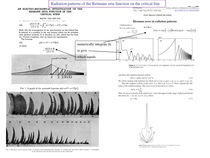
Radiation patterns of the Reimann zeta function on the critical line. numerically integrate fu to give which equals. Dipole array in formed in y direction a discrete number of dipoles are arranged into an antenna array with amplitudes given by a discrete f(u)

E N D
Radiation patterns of the Reimann zeta function on the critical line numerically integrate fu to give which equals
Dipole array in formed in y direction • a discrete number of dipoles are arranged into an antenna array with amplitudes given by a discrete f(u) • to save time and it is difficult to compute a real array of many dipoles since it requires too much computer memory and take too long, so just compute pattern of one dipole and then use the arraying facility to produce a simulated array pattern. This will be very similar to a real array provided the dipoles are relatively far apart in order to diminish mutual coupling. note: when I moved in y I called files _dx then after I computed I changed the heading to be dy to be consistent with what I actually did according to axis on left but plots still show _dx
To get f(u) text file run mathematica 'output fu text files for cst.nb' select range of points for fu. Mathematica then outputs the fu.txt file. In cst - dipole.cst run farfield array with fu.txt as amplitude weights . Use macro- array - set array farfield button then user defined amplitude and point to fu.txt. set array with number of points given by mathematica. Choose point separation x0 to give an array scaling about k x0 dt= say 40. This will give heights of the zeta zero up to about t=40. e.g u+-3 step 0.01 601 points du=0.01, dt=1/du=100 run array pattern in say x with dx separation between u points of 100mm. This dx *dt is called x0 by Berry. tmax=k*xo=k*dx*dt where k = 2pi/wavelength for 1GHz lambda=300mm so k = 2pi/300 ~0.02 therefore tmax = (0.02*100*100)=200 so can view radiation pattern nulls=zeta zero zeros for t up to 200. Export pattern into /maths/mathematica/zeta function and reiman hypothesis/array zeta zero analysis/cst van der pol edit pattern .txt so just 0 to 90. data-import into excel array_comp_1ghz. Read off angles of nulls (theta(n)) which can then be used to compute t(n) of the nth zeta zero from t(n)=sin theta(n)*k*dx*dt . Brian 14/2/2017
Cartesian Radiation Pattern at 1GHz: f(u) = ± 3, ± 5, ± 10, ± 15 step 0.01 dy=25mm should be dy theta (deg)
Cartesian Radiation Pattern at 1GHz: f(u) = ± 3, ± 5, ± 10, ± 15 step 0.01 dy=25mm Sixth Zeta Zero @45.817º First Zeta Zero @15.645º Zoomed into pattern nulls Tenth Zeta Zero @71.742º ‘pulling-off’ of zero near 90deg
3D Radiation Pattern at 1GHz: f(u) = ± 10 step 0.01 dx=25mm H Bomb Test
Cartesian Radiation Pattern at 1GHz: f(u) = ± 10 step 0.01 dx=25mm and dy=25mm Comparison dipole array in x and y tenth zero still at 71.3deg instead 71.7
Comparing CST Array Radiation Pattern of f(u) with discrete fourier transform of f(u) Dipole array Cartesian radiation pattern at 1GHz: f(u) = ± 3, ± 5, ± 10, ± 15 step 0.01 dy=25mm ANTENNA SOFTWARE f(u) range ±3, ±5, ±10, ±15 for u step = 0.01 deg matlab DFT Discrete Fourier Transform of f(u). Power spectrum g(t)= 10log10(FT[|f(u)|^2) = ± 3, ± 5, ± 10, ± 15 step 0.01
Comparing numerical integration of f(u) ±5step 1.047 with discrete (antenna sampled) fourier transform of f(u) ±5 step 0.01 (equivalent dt=1.047). Both power spectra loge(amp^2) t f(u) ±5 Purple is numerical integration - MATHEMATICA Blue is discrete FFT -MATLAB
Comparing numerical integration of f(u) ±10step 0.318 with discrete (antenna sampled) fourier transform of f(u) ±10 step 0.01 (equivalent dt=0.318). Both power spectra i.e loge(amp^2) t f(u) ±10 Purple is numerical integration - MATHEMATICA Blue is discrete FFT -MATLAB
Comparing numerical integration of f(u) ±15step 0.209 with discrete (antenna sampled) fourier transform of f(u) ±15 step 0.01 (equivalent dt=0.209). Both power spectra i.e loge(amp^2) t f(u) ±15 Purple is numerical integration - MATHEMATICA Blue is discrete FFT -MATLAB