Download

1 / 155
1.58k likes | 1.62k Views
Statistics in Medicine. Unit 4: Overview/Teasers. Overview. Probability distributions; expected value and variance; the binomial and normal distributions. Teaser 1, Unit 4. A 2012 Mega Millions lottery had a jackpot of $656 million ($474 immediate payout).

E N D
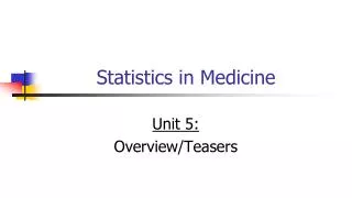
Statistics in Medicine Unit 4: Overview/Teasers
Overview • Probability distributions; expected value and variance; the binomial and normal distributions
Teaser 1, Unit 4 • A 2012 Mega Millions lottery had a jackpot of $656 million ($474 immediate payout). • Question I received: “If the odds of winning the Mega millions is 1 in 175,000,000 is there a significant statistical advantage in playing 100 quick picks rather than one? • “For a half-billion-with-a-B dollars it almost seems worth it.”
Teaser 2, Unit 4 Imagine that you are in a resource-poor area and you want to screen the population for a fairly rare disease. But the antibody test is prohibitively expensive. A clever cost-saving strategy is to pool the blood from multiple samples (using half of a person’s blood sample and saving the other half). If the pooled lot is negative, this saves n-1 tests. If it’s positive, then you go back and test each sample individually, requiring n+1 tests total. If a particular disease has a prevalence of 10% in a population, will the pooling strategy save you tests? If so, what’s the optimal number of samples to pool per lot?
Teaser 3, Unit 4 • Ten patients with wrinkles were photographed before and after treatment with a new anti-aging treatment. An independent dermatologist was able to distinguish the pre and post photographs for 9 out of the 10 subjects. • If the anti-aging treatment is completely ineffective, what’s the probability that the dermatologist could have gotten at least 9 right purely by lucky guessing?
Statistics in Medicine Module 1: Probability distributions
Probability function • Gives the probabilities of all possible outcomes. • A mathematical function that maps each possible outcome x to its probability p(x). • The probabilities must sum (or integrate) to 1.0.
Probability functions can be discrete or continuous • Discrete: can only take on certain values • Examples: Dead/alive, treatment/placebo, dice, whole numbers, counts, etc. • Continuous:can theoretically take on any value within a given range (has an infinite continuum of possible values). • Examples: blood pressure, weight, the speed of a car, the real numbers from 1 to 6
p(x) 1/6 x Discrete example: roll of a die 1 2 3 4 5 6
x p(x) 1 p(x=1)=1/6 2 p(x=2)=1/6 3 p(x=3)=1/6 4 p(x=4)=1/6 5 p(x=5)=1/6 6 p(x=6)=1/6 1.0 Probability mass function (pmf)
P(x) 1.0 5/6 2/3 1/2 1/3 1/6 x 1 2 3 4 5 6 Cumulative distribution function (CDF)
x P(x≤A) 1 P(x≤1)=1/6 2 P(x≤2)=2/6 3 P(x≤3)=3/6 4 P(x≤4)=4/6 5 P(x≤5)=5/6 6 P(x≤6)=6/6 Cumulative distribution function for a die
Recall: blood types Out of 100 donors . . . . . Source:AABB.ORG
Probability distribution for blood types (discrete function):
x 9 10 11 12 13 P(x) .3 .3 .2 .1 .1 Practice Problem: • The number of patients seen in the ER in any given hour is a random variable represented by x. The probability distribution for x is: Find the probability that in a given hour: a.exactly 13 patients arrive b.At least 12 patients arrive c.At most 11 patients arrive p(x=13)= .1 p(x12)= ( .1 +.1) = .2 p(x≤11)= (.3 +.3+.2) = .80
Important discrete distributions in medical research: • Binomial • Yes/no outcomes (dead/alive, treated/untreated, smoker/non-smoker, sick/well, etc.) • Poisson • Counts (e.g., how many cases of disease in a given area)
Continuous case • Any continuous mathematical function that integrates to 1 is a probability function. • The probabilities associated with continuous functions are just areas under the curve (integrals!). • Probabilities are given for a range of values, rather than a particular value.
Continuous case • For example, the exponential distribution is a continuous probability function, because the area under the curve is 1.0. • This function integrates to 1 (optional!):
p(x)=e-x 1 x Continuous case: “probability density function” (pdf) The probability that x is any exact particular value (such as 1.9976) is 0; we can only assign probabilities to possible ranges of x (=cumulative distribution function).
p(x)=e-x 1 The integral (optional!) x 1 2 Continuous case: Cumulative distribution function (CDF) Clinical example: Imagine that survival times after lung transplant roughly follow an exponential function. Then, the probability that a patient will die in the second year after surgery (between years 1 and 2) is 23%.
Optional extra material • Cumulative distribution function for the continuous case.
Cumulative distribution function As in the discrete case, we can specify the “cumulative distribution function” (CDF): The CDF here = P(x≤A)=
p(x) 1 x 2 Example
Practice Problem Suppose that survival drops off rapidly in the year following diagnosis of a certain type of advanced cancer. Suppose that the length of survival (or time-to-death) is a random variable that approximately follows an exponential distribution with parameter 2 (makes it a steeper drop off): What’s the probability that a person who is diagnosed with this illness survives a year?
Answer The probability of dying within 1 year can be calculated using the cumulative distribution function: Cumulative distribution function is: The chance of surviving past 1 year is: P(x≥1) = 1 – P(x≤1)
p(x) 1 x 1 We can see it’s a probability distribution because the area under the curve is 1: Example 2: Uniform distribution The uniform distribution: all values are equally likely. f(x)= 1 , for 1x 0
p(x) 1 x ¼ ½ 1 Example: Uniform distribution What’s the probability that x is between ¼ and ½? P(½ x ¼ )= ¼
p(x) ½ 0 1 x 1 Example: Uniform distribution What’s the probability that x is between 0 and ½? Clinical Research Example: When randomizing patients in an RCT, we often use a random number generator on the computer. These programs work by randomly generating a number between 0 and 1 (with equal probability of every number in between). Then a subject who gets X<.5 is control and a subject who gets X>.5 is treatment. P(½ x 0)= ½
Expected value and Variance • All probability distributions are characterized by an expected value (mean) and a variance (standard deviation squared).
One standard deviation from the mean () Mean () For example, bell-curve (normal) distribution:
Statistics in Medicine Module 2: Expected value
Expected value • Expected value is just the mean (µ) of a probability distribution. • It is a weighted average, calculated by weighting the value of each possible outcome by its probability. • Expected value helps us make informed decisions based on how we expect x to behave on-average over the long-run…( “frequentist” view).
Expected value, formally Discrete case: Continuous case:
x 9 10 11 12 13 P(x) .3 .3 .2 .1 .1 Example: expected value • Recall the following probability distribution of ER arrivals:
The probability (frequency) of each person in the sample is 1/n. A Sample Mean is a special case of Expected Value… Sample mean, for a sample of n subjects: =
Symbol Interlude • E(X) = µ • these symbols are used interchangeably
Expected Value • Expected value is an extremely useful concept for good decision-making!
Example: the lottery • The Lottery (also known as a tax on people who are bad at math…) • A certain lottery works by picking 6 numbers from 1 to 49. It costs $1.00 to play the lottery, and if you win, you win $2 million after taxes. If you play the lottery once, what are your expected winnings or losses?
x$ p(x) -1 .999999928 + 2 million 7.2 x 10--8 “49 choose 6” Out of 49 numbers, this is the number of distinct combinations of 6. Lottery Calculate the probability of winning in 1 try: The probability function (note, sums to 1.0):
x$ p(x) -1 .999999928 + 2 million 7.2 x 10--8 Expected Value The probability function Expected Value E(X) = P(win)*$2,000,000 + P(lose)*-$1.00 = 2.0 x 106 * 7.2 x 10-8+ .999999928 (-1) =.144 - .999999928 = -$.86 Negative expected value is never good! You shouldn’t play if you expect to lose money!
Expected Value If you play the lottery every week for 10 years, what are your expected winnings or losses? 520 x (-.86) = -$447.20
2012 record Mega Millions jackpot… • 2012 Mega Millions had a jackpot of $656 million ($474 immediate payout). • Question I received: “If the odds of winning the Mega millions is 1 in 175,000,000 is there a significant statistical advantage in playing 100 quick picks rather than one? • “For a half-billion-with-a-B dollars it almost seems worth it.”
x$ p(x) -1 . 999999994 + 500 million 6 × 10⁻⁹ Expected value for 1 ticket: • Chances of losing, 1 ticket: 1-1/175,000,000=99.9999994% Expected Value E(X) = P(win)*$500,000,000 + P(lose)*-$1.00 = 6.0 x 10-9 * 500,000,000+ .999999994 (-1) =+2
x$ p(x) -1 . 99999943 + 500 million 5.7× 10⁻⁷ Answer, 100 tickets: • Chances of losing, 100 tickets: 99.999943% Expected Value E(X) = P(win)*$500,000,000 + P(lose)*-$1.00 = 5.7 x 10-7 * 500,000,000+ .99999943 (-1) =+284
So… • One could make a case for playing! • You can work out that the expected payout only has to be >$176 million for expected value to be positive (for either 1 ticket or 100 tickets). • BUT…
BUT then consider the high chance of multiple winners! • When the jackpot is huge, lots of people play. The chance of multiple winners (who will share the jackpot) is quite high! • Assume 600 million tickets are sold, then the probability distribution here is (where x is the number of winners): • E(X)=0+1*.11+2*.19+3*.22+4*.19+5*.13+6*.07+7*.036+8*.015+9*.005+10*.002=3.4 • Therefore, the expected winnings if you win are actually 500 million/3.4=147 million
Not to mention taxes! • You can also assume that about half is going to be lost in taxes. • And, the fact is, you’re still going to lose with almost near certainty! • Probability 99.9999…%!
Gambling (or how casinos can afford to give so many free drinks…) A roulette wheel has the numbers 1 through 36, as well as 0 and 00. If you bet $1 that an odd number comes up, you win or lose $1 according to whether or not that event occurs. If random variable X denotes your net gain, X=1 with probability 18/38 and X= -1 with probability 20/38. E(X) = 1(18/38) – 1 (20/38) = -$.053 On average, the casino wins (and the player loses) 5 cents per game. The casino rakes in even more if the stakes are higher: E(X) = 10(18/38) – 10 (20/38) = -$.53 If the cost is $10 per game, the casino wins an average of 53 cents per game. If 10,000 games are played in a night, that’s a cool $5300.
Challenge Problem • Imagine that you are in a resource-poor area and you want to screen the population for a fairly rare disease. But the antibody test is prohibitively expensive. • A clever cost-saving strategy is to pool the blood from multiple samples (using half of a person’s blood sample and saving the other half). If the pooled lot is negative, this saves n-1 tests. If it’s positive, then you go back and test each sample individually, requiring n+1 tests total. • If a particular disease has a prevalence of 10% in a population, will the pooling strategy save you tests? If so, what’s the optimal number of samples to pool per lot? • Solve by “brute force” assuming you want to screen 100 people.