Download
1 / 74
750 likes | 767 Views
Discrete Probability. Chapter 7. Chapter Summary. Introduction to Discrete Probability Probability Theory Bayes ’ Theorem Expected Value and Variance. An Introduction to Discrete Probability. Section 7.1. Section Summary. Finite Probability

E N D
Discrete Probability Chapter 7
Chapter Summary • Introduction to Discrete Probability • Probability Theory • Bayes’ Theorem • Expected Value and Variance
An Introduction to Discrete Probability Section 7.1
Section Summary Finite Probability Probabilities of Complements and Unions of Events Probabilistic Reasoning
Probability of an Event Pierre-Simon Laplace (1749-1827) We first study Pierre-Simon Laplace’s classical theory of probability, which he introduced in the 18th century, when he analyzed games of chance. • We first define these key terms: • An experiment is a procedure that yields one of a given set of possible outcomes. • The sample space of the experiment is the set of possible outcomes. • An event is a subset of the sample space. • Here is how Laplace defined the probability of an event: Definition: If S is a finite sample space of equally likely outcomes, and E is an event, that is, a subset of S, then the probability of E is p(E) = |E|/|S|. • For every event E, we have 0≤p(E) ≤1. This follows directly from the definition because 0≤p(E) = |E|/|S| ≤ |S|/|S| ≤1, since 0 ≤ |E| ≤ |S|.
Applying Laplace’s Definition Example: An urn contains four blue balls and five red balls. What is the probability that a ball chosen from the urn is blue? Solution: The probability that the ball is chosen is 4/9 since there are nine possible outcomes, and four of these produce a blue ball. Example: What is the probability that when two dice are rolled, the sum of the numbers on the two dice is 7? Solution: By the product rule there are 62 = 36 possible outcomes. Six of these sum to 7. Hence, the probability of obtaining a 7 is 6/36 = 1/6.
Applying Laplace’s Definition Example: In a lottery, a player wins a large prize when they pick four digits that match, in correct order, four digits selected by a random mechanical process. What is the probability that a player wins the prize? Solution: By the product rule there are 104 = 10,000 ways to pick four digits. • Since there is only 1 way to pick the correct digits, the probability of winning the large prize is 1/10,000 = 0.0001. A smaller prize is won if only three digits are matched. What is the probability that a player wins the small prize? Solution: If exactly three digits are matched, one of the four digits must be incorrect and the other three digits must be correct. For the digit that is incorrect, there are 9 possible choices. Hence, by the sum rule, there a total of 36 possible ways to choose four digits that match exactly three of the winning four digits. The probability of winning the small price is 36/10,000 = 9/2500 = 0.0036.
Applying Laplace’s Definition Example: There are many lotteries that award prizes to people who correctly choose a set of six numbers out of the first n positive integers, where n is usually between 30 and 60. What is the probability that a person picks the correct six numbers out of 40? Solution: The number of ways to choose six numbers out of 40 is C(40,6) = 40!/(34!6!) = 3,838,380. Hence, the probability of picking a winning combination is 1/ 3,838,380 ≈ 0.00000026. Can you work out the probability of winning the lottery with the biggest prize where you live?
Applying Laplace’s Definition Example: What is the probability that the numbers 11, 4, 17, 39, and 23 are drawn in that order from a bin with 50 balls labeled with the numbers 1,2, …, 50 if • The ball selected is not returned to the bin. • The ball selected is returned to the bin before the next ball is selected. Solution: Use the product rule in each case. a)Sampling without replacement: The probability is 1/254,251,200 since there are 50 ∙49 ∙47 ∙46 = 254,251,200 ways to choose the five balls. b) Sampling with replacement: The probability is 1/505 = 1/312,500,000 since 505= 312,500,000.
The Probability of Complements and Unions of Events Theorem 1: Let E be an event in sample space S. The probability of the event = S − E, the complementary event of E, is given by Proof: Using the fact that | | = |S| − |E|,
The Probability of Complements and Unions of Events Example: A sequence of 10 bits is chosen randomly. What is the probability that at least one of these bits is 0? Solution: Let E be the event that at least one of the 10 bits is 0. Then is the event that all of the bits are 1s. The size of the sample space S is 210. Hence,
The Probability of Complements and Unions of Events Theorem 2: Let E1andE2 be events in the sample space S. Then Proof: Given the inclusion-exclusion formula from Section 2.2, |A ∪ B| = |A| + | B| − |A ∩ B|, it follows that
The Probability of Complements and Unions of Events Example: What is the probability that a positive integer selected at random from the set of positive integers not exceeding 100 is divisible by either 2 or 5? Solution: Let E1be the event that the integer is divisible by 2 andE2 be the event that it is divisible 5? Then the event that the integer is divisible by 2 or 5 is E1 ∪ E2 and E1 ∩ E2 is the event that it is divisible by 2 and 5. It follows that: p(E1 ∪ E2) = p(E1) + p(E2) – p(E1 ∩ E2) = 50/100 + 20/100 − 10/100 = 3/5.
1 2 3 Monty Hall Puzzle (This is a notoriously confusing problem that has been the subject of much discussion . Do a web search to see why!) Example: You are asked to select one of the three doors to open. There is a large prize behind one of the doors and if you select that door, you win the prize. After you select a door, the game show host opens one of the other doors (which he knows is not the winning door). The prize is not behind the door and he gives you the opportunity to switch your selection. Should you switch? Solution: You should switch. The probability that your initial pick is correct is 1/3. This is the same whether or not you switch doors. But since the game show host always opens a door that does not have the prize, if you switch the probability of winning will be 2/3, because you win if your initial pick was not the correct door and the probability your initial pick was wrong is 2/3.
Probability Theory Section 7.2
Section Summary Assigning Probabilities Probabilities of Complements and Unions of Events Conditional Probability Independence Bernoulli Trials and the Binomial Distribution Random Variables The Birthday Problem Monte Carlo Algorithms The Probabilistic Method (not currently included in the overheads)
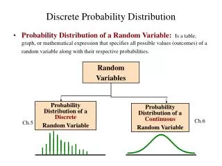
Assigning Probabilities Laplace’s definition from the previous section, assumes that all outcomes are equally likely. Now we introduce a more general definition of probabilities that avoids this restriction. • Let S be a sample space of an experiment with a finite number of outcomes. We assign a probability p(s) to each outcome s, so that: i.0 ≤ p(s) ≤ 1 for each sÎ S ii. • The function p from the set of all outcomes of the sample space S is called a probability distribution.
Assigning Probabilities Example: What probabilities should we assign to the outcomes H(heads) and T (tails) when a fair coin is flipped? What probabilities should be assigned to these outcomes when the coin is biased so that heads comes up twice as often as tails? Solution: We have p(H) = 2p(T). Because p(H) + p(T) = 1, it follows that 2p(T) + p(T) = 3p(T) = 1. Hence, p(T) = 1/3 andp(H) = 2/3.
Uniform Distribution Definition: Suppose that S is a set with n elements. The uniform distribution assigns the probability 1/n to each element of S. (Note that we could have used Laplace’s definition here.) Example: Consider again the coin flipping example, but with a fair coin. Now p(H) = p(T) = 1/2.
Probability of an Event Definition: The probability of the event E is the sum of the probabilities of the outcomes in E. Note that now no assumption is being made about the distribution.
Example Example: Suppose that a die is biased so that 3 appears twice as often as each other number, but that the other five outcomes are equally likely. What is the probability that an odd number appears when we roll this die? Solution: We want the probability of the event E = {1,2,3}. We have p(3) =2/7 and p(1) =p(2) =p(4) =p(5) =p(6) =1/7. Hence, p(E) = p(1) +p(3) +p(5) = 1/7 + 2/7 + 1/7 = 4/7.
Probabilities of Complements and Unions of Events Complements: still holds. Since each outcome is in either E or , but not both, Unions: also still holds under the new definition.
Combinations of Events see Exercises 36and37for the proof Theorem: If E1, E2, … is a sequence of pairwise disjoint events in a sample space S, then
Conditional Probability Definition: Let E and F be events with p(F) > 0. The conditional probability of E given F, denoted by P(E|F), is defined as: Example: A bit string of length four is generated at random so that each of the 16 bit strings of length 4 is equally likely. What is the probability that it contains at least two consecutive 0s, given that its first bit is a 0? Solution: Let E be the event that the bit string contains at least two consecutive 0s, and F be the event that the first bit is a 0. • Since E⋂F = {0000, 0001, 0010, 0011, 0100}, p(E⋂F)=5/16. • Because 8 bit strings of length 4 start with a 0, p(F) = 8/16= ½. Hence,
Conditional Probability Example: What is the conditional probability that a family with two children has two boys, given that they have at least one boy. Assume that each of the possibilities BB, BG, GB, and GG is equally likely where B represents a boy and G represents a girl. Solution: Let E be the event that the family has two boys and let F be the event that the family has at least one boy. Then E = {BB}, F = {BB, BG, GB}, and E⋂F = {BB}. • It follows that p(F) = 3/4 and p(E⋂F)=1/4. Hence,
Independence p(E⋂F) = p(E)p(F). p(E) = p(F) = 8/16 = ½. Definition: The events E and F are independent if and only if Example: Suppose E is the event that a randomly generated bit string of length four begins with a 1 and F is the event that this bit string contains an even number of 1s. Are E and F independent if the 16 bit strings of length four are equally likely? Solution: There are eight bit strings of length four that begin with a 1, and eight bit strings of length four that contain an even number of 1s. • Since the number of bit strings of length 4 is 16, • Since E⋂F = {1111, 1100, 1010, 1001}, p(E⋂F) = 4/16=1/4. We conclude that E and F are independent, because p(E⋂F) =1/4 = (½) (½)= p(E)p(F)
Independence Example: Assume (as in the previous example) that each of the four ways a family can have two children (BB, GG, BG,GB) is equally likely. Are the events E, that a family with two children has two boys, and F, that a family with two children has at least one boy, independent? Solution: Because E = {BB}, p(E) = 1/4. We saw previously that that p(F) = 3/4 and p(E⋂F)=1/4. The events E and F are not independent since p(E) p(F) = 3/16 ≠1/4= p(E⋂F).
Pairwise and Mutual Independence Definition: The events E1, E2, …, En are pairwise independent if and only if p(Ei⋂Ej) = p(Ei) p(Ej) for all pairs i and j with i≤ j ≤ n. The events are mutually independent if whenever ij, j = 1,2,…., m, are integers with 1 ≤ i1 < i2 <∙∙∙ <im≤ n and m≥ 2.
James Bernoulli (1854 – 1705) Bernoulli Trials Definition: Suppose an experiment can have only two possible outcomes, e.g., the flipping of a coin or the random generation of a bit. • Each performance of the experiment is called a Bernoulli trial. • One outcome is called a success and the other a failure. • If p is the probability of success and q the probability of failure, then p + q = 1. • Many problems involve determining the probability of k successes when an experiment consists of n mutually independent Bernoulli trials.
Bernoulli Trials Example: A coin is biased so that the probability of heads is 2/3. What is the probability that exactly four heads occur when the coin is flipped seven times? Solution: There are 27 = 128 possible outcomes. The number of ways four of the seven flips can be heads is C(7,4). The probability of each of the outcomes is (2/3)4(1/3)3 since the seven flips are independent. Hence, the probability that exactly four heads occur is C(7,4) (2/3)4(1/3)3 = (35∙ 16)/27 = 560/2187.
Probability of k Successes in n Independent Bernoulli Trials. Theorem 2: The probability of exactly k successes in n independent Bernoulli trials, with probability of success p and probability of failure q = 1− p, is C(n,k)pkqn−k. Proof: The outcome of n Bernoulli trials is an n-tuple (t1,t2,…,tn), where each isti either S (success) or F (failure). The probability of each outcome of n trials consisting of k successes and k−1 failures (in any order) is pkqn−k. Because there are C(n,k) n-tuples of Ss and Fs that contain exactly k Ss, the probability of k successes is C(n,k)pkqn−k. We denote by b(k:n,p) the probability of k successes in n independent Bernoulli trials with p the probability of success. Viewed as a function of k, b(k:n,p) is the binomial distribution. By Theorem 2, b(k:n,p) = C(n,k)pkqn−k.
Random Variables Definition: A random variable is a function from the sample space of an experiment to the set of real numbers. That is, a random variable assigns a real number to each possible outcome. A random variable is a function. It is not a variable, and it is not random! In the late 1940s W. Feller and J.L. Doob flipped a coin to see whether both would use “random variable” or the more fitting “chance variable.” Unfortunately, Feller won and the term “random variable” has been used ever since.
Random Variables Definition: The distribution of a random variable X on a sample space S is the set of pairs (r, p(X = r)) for all r∊X(S), where p(X = r) is the probability that X takes the value r. Example: Suppose that a coin is flipped three times. Let X(t) be the random variable that equals the number of heads that appear when t is the outcome. Then X(t) takes on the following values: X(HHH) = 3, X(TTT) = 0, X(HHT) = X(HTH) = X(THH) = 2, X(TTH) = X(THT) = X(HTT) = 1. Each of the eight possible outcomes has probability 1/8. So, the distribution of X(t) is p(X = 3) = 1/8, p(X = 2) = 3/8, p(X = 1) = 3/8, and p(X = 0) = 1/8.
The Famous Birthday Problem • The puzzle of finding the number of people needed in a room to ensure that the probability of at least two of them having the same birthday is more than ½ has a surprising answer, which we now find. Solution: We assume that all birthdays are equally likely and that there are 366 days in the year. First, we find the probability pn that at least two of n people have different birthdays. Now, imagine the people entering the room one by one. The probability that at least two have the same birthday is 1−pn . • The probability that the birthday of the second person is different from that of the first is 365/366. • The probability that the birthday of the third person is different from the other two, when these have two different birthdays, is 364/366. • In general, the probability that the jth person has a birthday different from the birthdays of those already in the room, assuming that these people all have different birthdays, is (366 − (j− 1))/366 = (367 − j)/366. • Hence, pn = (365/366)(364/366)∙∙∙ (367 − n)/366. • Therefore , 1− pn = 1−(365/366)(364/366)∙∙∙ (367 − n)/366. Checking various values for n with computation help tells us that for n = 22, 1− pn≈0.457, and for n = 23, 1− pn≈0.506. Consequently, a minimum number of 23 people are needed so that that the probability that at least two of them have the same birthday is greater than 1/2.
Monte Carlo Algorithms • Algorithms that make random choices at one or more steps are called probabilistic algorithms. • Monte Carlo algorithms are probabilistic algorithms used to answer decision problems, which are problems that either have “true” or “false” as their answer. • A Monte Carlo algorithm consists of a sequence of tests. For each test the algorithm responds “true” or ‘unknown.’ • If the response is “true,” the algorithm terminates with the answer is “true.” • After running a specified sequence of tests where every step yields “unknown”, the algorithm outputs “false.” • The idea is that the probability of the algorithm incorrectly outputting “false” should be very small as long as a sufficient number of tests are performed.
Probabilistic Primality Testing • Probabilistic primality testing (see Example 16in text) is an example of a Monte Carlo algorithm, which is used to find large primes to generate the encryption keys for RSA cryptography (as discussed in Chapter 4). • An integer n greater than 1 can be shown to be composite (i.e., not prime) if it fails a particular test (Miller’s test), using a random integer b with 1 < b < n as the base. But if n passes Miller’s test for a particular base b, it may either be prime or composite. The probability that a composite integer passes n Miller’s test is for a random b, is less that ¼. • So failing the test, is the “true” response in a Monte Carlo algorithm, and passing the test is “unknown.” • If the test is performed k times (choosing a random integer b each time) and the number n passes Miller’s test at every iteration, then the probability that it is composite is less than (1/4)k. So for a sufficiently, large k, the probability that n is composite even though it has passed all k iterations of Miller’s test is small. For example, with 10 iterations, the probability that n is composite is less than 1 in 1,000,000.
Bayes’ Theorem Section 7.3
Section Summary Bayes’ Theorem Generalized Bayes’ Theorem Bayesian Spam Filters A.I. Applications (optional, not currently included in the overheads)
Motivation for Bayes’ Theorem • Bayes’ theorem allows us to use probability to answer questions such as the following: • Given that someone tests positive for having a particular disease, what is the probability that they actually do have the disease? • Given that someone tests negative for the disease, what is the probability, that in fact they do have the disease? • Bayes’ theorem has applications to medicine, law, artificial intelligence, engineering, and many diverse other areas.
Thomas Bayes (1702-1761) Bayes’ Theorem Bayes’ Theorem: Suppose that E and F are events from a sample space S such that p(E)≠0 and p(F) ≠0. Then: Example: We have two boxes. The first box contains two green balls and seven red balls. The second contains four green balls and three red balls. Bob selects one of the boxes at random. Then he selects a ball from that box at random. If he has a red ball, what is the probability that he selected a ball from the first box. • Let E be the event that Bob has chosen a red ball and F be the event that Bob has chosen the first box. • By Bayes’ theorem the probability that Bob has picked the first box is:
Derivation of Bayes’ Theorem continued → Recall the definition of the conditional probability p(E|F): From this definition, it follows that: ,
Derivation of Bayes’ Theorem On the last slide we showed that , Equating the two formulas for p(E F) shows that Solving for p(E|F) and for p(F|E) tells us that , continued →
Derivation of Bayes’ Theorem On the last slide we showed that: Note that since because and By the definition of conditional probability, Hence,
Applying Bayes’ Theorem Example: Suppose that one person in 100,000 has a particular disease. There is a test for the disease that gives a positive result 99% of the time when given to someone with the disease. When given to someone without the disease, 99.5% of the time it gives a negative result. Find • the probability that a person who test positive has the disease. • the probability that a person who test negative does not have the disease. • Should someone who tests positive be worried?
Applying Bayes’ Theorem Can you use this formula to explain why the resulting probability is surprisingly small? So, don’t worry too much, if your test for this disease comes back positive. Solution: Let D be the event that the person has the disease, and E be the event that this person tests positive. We need to compute p(D|E) from p(D), p(E|D), p( E |),p( ).
Applying Bayes’ Theorem So, the probability you have the disease if you test negative is • What if the result is negative? • So, it is extremely unlikely you have the disease if you test negative.
Generalized Bayes’ Theorem Exercise 17 asks for the proof. Generalized Bayes’ Theorem: Suppose that E is an event from a sample space S and that F1, F2, …, Fn are mutually exclusive events such that Assume that p(E) ≠ 0 for i = 1, 2, …, n. Then
Bayesian Spam Filters • How do we develop a tool for determining whether an email is likely to be spam? • If we have an initial set B of spam messages and set G of non-spam messages. We can use this information along with Bayes’ law to predict the probability that a new email message is spam. • We look at a particular word w, and count the number of times that it occurs in B and in G; nB(w) and nG(w). • Estimated probability that an email containing w is spam: p(w) = nB(w)/|B| • Estimated probability that an email containing w is spam: q(w) = nG(w)/|G| continued→
Bayesian Spam Filters Assuming that it is equally likely that an arbitrary message is spam and is not spam; i.e., p(S) = ½. Note: If we have data on the frequency of spam messages, we can obtain a better estimate for p(s). (See Exercise 22.) Using our empirical estimates of p(E | S) and p(E |`S). r(w) estimates the probability that the message is spam. We can class the message as spam if r(w) is above a threshold. Let S be the event that the message is spam, and E be the event that the message contains the word w. Using Bayes’ Rule,
Bayesian Spam Filters We class the message as spam and reject the email! Example: We find that the word “Rolex” occurs in 250 out of 2000 spam messages and occurs in 5 out of 1000 non-spam messages. Estimate the probability that an incoming message is spam. Suppose our threshold for rejecting the email is 0.9. Solution: p(Rolex) = 250/2000 =.0125 and q(Rolex) = 5/1000 = 0.005.