Download
1 / 37
370 likes | 397 Views
Demand-Side Equilibrium: Multiplier Analysis A definite ratio, to be called the Multiplier, can be established between income and investment. JOHN MAYNARD KEYNES Asst. Prof. Dr. Serdar AYAN. The Meaning of Equilibrium GDP.

E N D
Demand-Side Equilibrium: Multiplier Analysis A definite ratio, to be called the Multiplier, can be established between income and investment. JOHN MAYNARD KEYNES Asst. Prof. Dr. Serdar AYAN
The Meaning of Equilibrium GDP • GDP cannot be at its equilibrium if total spending differs from the value of output. • If spending exceeds output, inventories fall and firms increase production. • If output exceeds spending, inventories rise and firms reduce production.
Rest of the World Firms (produce the domestic product) Income (Y) Gross National FIGURE 1. The Circular Flow Diagram Financial System C + I 3 Investment (I) Consumption (C) 2 C + I + G Imports (IM) Purchases (G) Saving (S) Exports (X) Investors 4 Government C + I + G + Consumers 1 Government (X – IM) Disposable 5 Taxes Transfers 6 Income (DI) .
The Meaning of Equilibrium GDP • The equilibrium level of GDP on the demand side is the one at which total spending equals production. • In such a situation, firms find their inventories remaining at desired levels, so there is no incentive to change output or prices.
The Mechanics of Income Determination • Constructing the total expenditure schedule • Expenditure Schedule = table showing the relationship between GDP and total spending • Induced Investment = the part of investment spending that rises when GDP rises, and falls when GDP falls.
C + I + G C + I + G + ( X – I M ) X – IM = –$100 C + I G = $1,300 C I = $900 FIGURE 2.Construction of the Expenditure Schedule 6,100 6,000 Real Expenditure 4,800 3,900 5,200 5,600 6,000 6,400 6,800 7,200 Real GDP .
The Mechanics of Income Determination • Both the expenditure table and the corresponding “income-expenditure diagram” or “45 degree line diagram” show the equilibrium level of GDP. • All other levels of GDP are disequilibrium points, at which GDP will move in the direction of the equilibrium.
Output exceeds spending 45° C + I + G + ( X – I M ) E Equilibrium Spending exceeds output FIGURE 3.Income-Expenditure Diagram 7,200 6,800 6,400 6,000 Real Expenditure 5,600 5,200 4,800 0 4,800 5,200 5,600 6,000 6,400 6,800 7,200 Real GDP
The Aggregate Demand Curve • price level consumption • Therefore, price level total expenditures and equilibrium GDP • Therefore, price level equilibrium level of real aggregate quantity demanded
45 45 C + I + G + ( X – I M ) 2 E 2 C + I + G + ( X – I M ) 0 E C + I + G + ( X – I M ) 0 0 E 0 C + I + G + ( X – I M ) 1 E 1 45 45 Y Y Y Y 1 0 0 2 ( a) ( b) Rise in Pric e Level Fall in Pric e Level FIGURE 4.The Effect of the Price Level on Equilibrium AD Real Expenditure Real Expenditure Real GDP Real GDP
The Aggregate Demand Curve • The negatively-sloped aggregate demand curve shows all the equilibria of price levels and GDP. • Remember that any income-expenditure diagram is drawn for a specific price level.
E P 1 1 E P 0 0 E 2 P 2 Y Y Y 1 0 2 FIGURE 5.The Aggregate Demand Curve Price Level Real GDP
Demand-Side Equilibrium and Full Employment • Equilibrium GDP may not = full-employment GDP. • Recessionary gap: amount by which equilibrium GDP < potential GDP • Inflationary gap: amount by which equilibrium GDP > potential GDP
Potential GDP 45° F C + I + G + ( X – I M ) E B Recessionary gap 45° FIGURE 6.A Recessionary Gap Real Expenditure 6,000 7,000 Real GDP
Potential 45° GDP Inflationary gap E B C + I + G + ( X – I M ) F 45° FIGURE 7.An Inflationary Gap Real Expenditure 7,000 8,000 Real GDP
The Coordination of Saving and Investment • Equilibrium GDP = full employment only if saving out of full-employment incomes = investment • Savers are not the same people as investors, so it is unlikely that this condition will hold.
Firms (produce the domestic product) FIGURE 8.A Simplified Circular Flow Financial System C + I Consumption (C) Investment (I) 2 Saving (S) Investors C + I Consumers 1 3 Y
Changes on the Demand Side: Multiplier Analysis • Multiplier = ratio of the change in equilibrium GDP (Y) divided by the original change in spending that caused the change in GDP
Changes on the Demand Side: Multiplier Analysis • Demystifying the Multiplier: How It Works • The multiplier is greater than 1 because one person’s spending is another person’s income. • spending income • A portion of the increase in income is spent on consumption, creating more income, which in turn creates more consumption spending, and so on.
The Consumption Function and the Marginal Propensity to Consume • Marginal Propensity to Consume = consumption disposable income
FIGURE 10.How the Multiplier Builds $4.0 3.0 Cumulative Spending Total 2.0 1.0 0 2 4 6 8 10 15 20 Spending Round
Changes on the Demand Side: Multiplier Analysis • Algebraic Statement of the Multiplier • Multiplier = 1 (1 - MPC) • The MPC has been estimated to be about 0.9, implying that the multiplier is 10. • In fact, the multiplier is < 2.
Changes on the Demand Side: Multiplier Analysis • Algebraic Statement of the Multiplier • Factors that reduce the size of the multiplier • International trade • Inflation • Income taxation • Financial system
The Multiplier Is a General Concept • An autonomous change in consumer spending (caused by something other than an increase in income) shifts the consumption function and has a multiplier effect, just the same as a change in I does.
The Multiplier Is a General Concept • Other multiplier effects: • A change in G has the same multiplier effect as a change in I or a change in autonomous C. • The multiplier effect of a change in (X - IM) is the same as for the other components of spending. • Consequently, trade links the GDPs of the major economies.
The Multiplier Is a General Concept • GDP in a foreign country its imports, a portion of which are exports from the Turkiye. • The growth in U.S. exports has a multiplier effect, raising GDP in the Turkiye. • Booms and recessions tend to be transmitted across national borders.
The Multiplier and the Aggregate Demand Curve • autonomous spending horizontal shift of the AD curve by an amount given by the oversimplified multiplier formula.
45 ° C + I + G + (X – I M ) 1 E C + I + G + ( X – I M ) 1 0 $200 billion E 0 6,000 6,800 D D 0 1 E E 0 1 D ( I = $1,100) 1 D ( I = $900) 0 6,800 FIGURE 12.Two Views of the Multiplier Real Expenditure 0 Price Level 100 6,000 Real GDP
The Simple Algebra of Income Determination and the Multiplier
Simple Algebra of Income Determination & Multiplier • All of the relationships discussed can be represented in simple algebra.
Simple Algebra of Income Determination & Multiplier • Consumption function: C = a + b(DI) • Positive linear relationship between C and DI • a = autonomous consumption, determined by factors aside from DI • b = marginal propensity to consume = C/ DI • b(DI) = induced consumption, determined by DI
Simple Algebra of Income Determination & Multiplier • Equilibrium Y = C + I + G + (X - IM), so Equilibrium Y = a + b(DI) + I + G + (X - IM) • Since DI = Y - T, Equilibrium Y = a + b(Y - T) + I + G + (X - IM) • Therefore Equilibrium Y = a + bY - bT + I + G + (X - IM)
Simple Algebra of Income Determination & Multiplier • Then solve for Y: Equilibrium Y = [a - bT + I + G + (X - IM)] / (1 - b)