Large Scale Structure at High Redshift in the GOODS Field

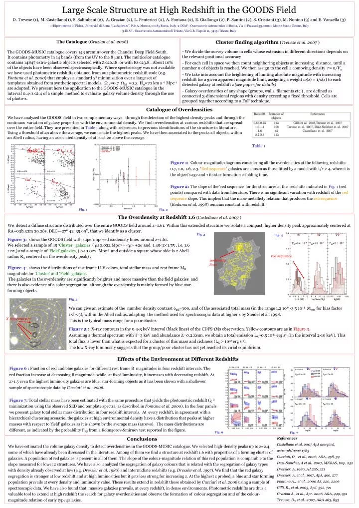
1. Large Scale Structure at High Redshift in the GOODS Field D. Trevese (1),M. Castellano(1), S. Salimbeni (2), A. Grazian (2), L. Pentericci (2), A. Fontana (2), E. Giallongo (2), P. Santini (2), S. Cristiani (3), M. Nonino (3) and E. Vanzella (3) 1--Dipartimento di Fisica, Università di Roma “La Sapienza”, P.le A. Moro 2, 00185 Roma, Italy 2-INAF - Osservatorio Astronomico di Roma, Via di Frascati 33, 00040 Monte Porzio Catone, Italy3-INAF - Osservatorio Astronomico di Trieste, Via G.B. Tiepolo 11, 34131 Trieste, Italy Cluster finding algorithm (Trevese et al. 2007) - We divide the survey volume in cells whose extension in different directions depends on the relevant positional accuracy - For each cell in space we then count neighboring objects at increasing distance, until a number n of objects is reached. We then assign to the cell a comoving density r= n/Vn - We take into account the brightening of limiting absolute magnitude with increasing redshift for a given apparent magnitude limit, assigning a weight w(z) = 1/s(z) to each detected galaxy at redshift z (see paper for details) - Galaxy overdensities of any shape (groups, walls, filaments etc.), are defined as connected 3-dimensional regions with density exceeding a fixed threshold. Cells are grouped together according to a FoF technique. The Catalogue (Grazian et al. 2006) The GOODS-MUSIC catalogue covers 143 arcmin2 over the Chandra Deep Field South. It contains photometry in 14 bands (from the UV to the 8 mm). The multicolor catalogue contains 14847 extra-galactic objects selected with Z<26.18  or with Ks<23.8 . About 10% of the objects have been observed spectroscopically. Where spectroscopy was not available we have used photometric redshifts obtained from our photometric redshift code (e.g. Fontana et al. 2000) that employs a standard c2 minimization over a large set of templates obtained from synthetic spectral models. WL=0.7  WM  =0.3  H0=70 km s -1 Mpc-1 are adopted. We present here the application to the GOODS-MUSIC catalogue in the interval 0.4<z<2.4 of a simple method to evaluate galaxy volume density through the use of photo-z. Catalogue of Overdensities We have analyzed the GOODS field in two complementary ways: through the detection of the highest density peaks and through the continuos variation of galaxy properties with the environmental density. We find overedensities at various redshifts that are spread over the entire field. They are presented in Table 1 along with references to previous identifications of the structure in literature. Using a threshold of 4s above the average, we can isolate the highest peaks. We have then associated to the peaks all objects, within an Abell radius, having an associated density of at least 2s above the average. Table 1 Figure 1: Colour-magnitude diagrams considering all the overdensities at the following redshifts: 0.7, 1.0, 1.6, 2.3. ‘Red sequence’ galaxies are chosen as those fitted by a model with t/t > 4, where t is the object’s age and t its star-formation e-folding time. Figure 2: The slope of the 'red sequence' for the structures at the redshifts indicated in Fig. 1 (red points) compared with data from literature. There is no significant variation with redshift of the red sequence slope. This implies that the mass-metallicty relation that produces the red sequence (Kodama et al. 1998) remains constant with redshift. Fig. 1 Fig. 2 The Overdensity at Redshift 1.6 (Castellano et al. 2007) We detect a diffuse structuredistributed over the entire GOODS fieldaround z=1.61. Within this extended structure we isolate a compact, higher density peakapproximately centered at RA=03h 32m 29.28s, DEC=-27° 42' 35.99'‘, that we identify as a cluster. Fig. 3 Fig. 4 Figure 3: shows the GOODS field with superimposed isodensity linesaround z=1.61. We selected a sample of 45 ‘Cluster ’ galaxies (0.022 Mpc-3= <> +2 and 1.45<z<1.75 , i.e. 1.6 2z) and a sample of ‘Field’ galaxies, (<0.022 Mpc-3 and outside a square whose side is 2 Abell radius RAcentered on the overdensity peak) . Figure 4:shows the distributions of rest frame U-V colors, total stellar mass and rest frame MB magnitude for ‘Cluster’ and ‘Field’ galaxies. The galaxies in the overdensity are significantly brighter and more massive than the field galaxies and there is also evidence of a color segregation, although the overdensity is mainly formed by blue star-forming objects. red sequence isodensity lines Fig. 5 We can give an estimate of the number density contrast gal300, and of the associated total mass (in the range 1.2 1014-3.5 1014Msun for bias factor 1<b<3), within the Abell radius, adapting the method used for spectroscopic data at higher z by Steidel et al. 1998. This is the typical mass range for a poor cluster. Figure 5 : X-ray contours in the 0.4-3 keV interval (black lines) of the CDFS 1Ms observation. Yellow contours are as in Figure 3. Assuming a thermal spectrum with T=3 keV and abundance Z=0.2 Zsun, we obtain a total emission LX0.5 1043 erg s-1 (in the interval 2-10 keV). This total flux is lower than what is expected for a cluster of this mass and richness (LX> 1043 erg s-1). The low X-ray luminosity suggests that the group/poor cluster has not yet reached its virial equilibrium. X-ray contours Effects of the Environment at Different Redshifts Figure 6 : Fraction of red and blue galaxies for different rest frame B magnitudes in four redshift intervals. The red fraction increase at decreasing B magnitude, while, at fixed luminosity, it increases with decreasing redshift. At z>1.5 even the highest luminosity galaxies are blue, star-forming objects as it has been shown with a shallower sample of spectroscopic data by Cucciati et al., 2006. Figure 7: Total stellar mass have been estimated with the same procedure that yields the photometric redshift (c 2 minimization using the observed SED and template spectra, as described in Fontana et al. 2000). In the four panels we present galaxy total stellar mass distribution in four redshift intervals. At every redshift, in agreement with a hierarchical clustering scenario, the galaxies at high environmental density have a distribution that peaks at higher masses with respect to 'field' galaxies as it is shown by the average mass (arrows). The mass distributions are different, as indicated by the probability PKS from a Kolmgorov-Smirnov test reported in the figure. Fig. 6 Fig. 7 Conclusions We have estimated the volume galaxy density to detect overdensities in the GOODS-MUSIC catalogue. We selected high-density peaks up to z=2.4, some of which have already been discussed in the literature. Among of them we find a structure at redshift 1.6 with properties of a forming cluster of galaxies. A population of red galaxies is present in all of them. The slope of the colour-magnitude relation of this red population is comparable to the slope measured for lower z structures. We have also analyzed the segregation of galaxy colours that is related with the segregation of galaxy types with density already observed at low (e.g. Dressler et al. 1980) and intermidiate redshifts (e.g. Dressler et al. 1997). We find that the red galaxy segregation is stronger at low redshift and at high luminosities but it gets less strong for increasing z. At the highest z probed, a blue and star forming population prevails at every density and luminosity value. These results extend in redshift those obtained by Cucciati et al. 2006 using a sample of spectroscopic data. We have also found that massive galaxies prevails, at every redshift, in dense environments. Photometric redshifts are thus a valuable tool to extend at high redshift the search for galaxy overdensities and observe the formation of colour segregation and of the colour-magnitude relation of early type galaxies. References Castellano et al. 2007 ApJ accepted, astro-ph/0707.1783 Cucciati, O., et al., 2006, A&A, 458, 39 Dıaz-Sanchez, A et al. 2007, MNRAS, tmp, 252 Dressler, A. 1980, AJ 236, 351 Dressler, A. et al., 1997, ApJ, 490, 577 Fontana A., et al., 2000 AJ, 220, 2206 Gilli, R., et al. 2003, ApJ, 592, 721 Grazian A., et al., Apr. 2006, A&A, 449, 951 Trevese, D., et al. 2007, A&A 463, 853