Download
1 / 35
370 likes | 612 Views
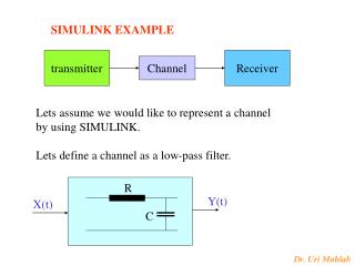
SIMULINK EXAMPLE. transmitter. Receiver. Channel. Lets assume we would like to represent a channel by using SIMULINK. Lets define a channel as a low-pass filter. R. Y(t). X(t). C. In the time domain we get :. X(t). Y(t). R. C. Simulation goals. H(z). source. scope. In. Out.

E N D
SIMULINK EXAMPLE transmitter Receiver Channel Lets assume we would like to represent a channel by using SIMULINK. Lets define a channel as a low-pass filter. R Y(t) X(t) C
X(t) Y(t) R C Simulation goals H(z) source scope In Out Definitions before we start to build the model: 1 - Drawing the icon picture F cut-off = [Hz]
2 – User guide window T-sample R C 3 -Look under mask T-sample In R C 4 – S function
METHOD 1
Step – 1 -Setup the working environment 1) Define the relevant path 2) Building the block model by: File new model
system Step – 2 -input ports Build input ports in out S-function
Step - 3 - Operation with Mask editor called “Edit Mask ” Icon on the Block Click right mouth This is the frame where you build the windows guide ICON PARAMETERS Init.. Documentation Prompt VariableType Tsampleedit Redit Cedit Connecting the block constant to the real parameters Mask type Mask description
Units “Normalized 01 11 10 00 Step – 3-1 – draw icon 0.2 0.5 0.85 0.80 0.75 R C fprintf(‘Fcutoff=%1.2f’,1/RC) %plot([x],[y]) plot([0,0.2],[0.8,0.8]) plot ([0.2, 0.2, 0.5, 0.5, 0.2],[0.75,0.85,0.85,0.75,0.75]) Plot([0.5,1],[0.8,0.8])
Step – 4 -Start with S - function S – function contains the name of the program and users parameters Choose the S-Function from the “User Define function” library S-function name should be the same as the name of the file.m
Step – 4-1: S-function returns inputs Function(sys, xo, str, ts)=s_function_name(t,x,u,flag,parameters) s_function_name Gets: t- running time x – state variable u- input signal flag – s_function status flag Returns sys – model parament array x0 – initial state conditions str – state ordering string ts – sampling time Model_name <> S-Function name function [sys,x0,str,ts] = sfunc_DiffequLPF(t,x,u,flag,Tsample,R,C)
The model should look like : Double click
Step – 4:1 – Defining the S-function a) Initialization – setup number of input and outputs function [sys,x0,str,ts]=mdlInitializeSizes % call simsizes for a sizes structure, fill it in and convert it to a % sizes array. % Note that in this example, the values are hard coded. This is not a % recommended practice as the characteristics of the block are typically % defined by the S-function parameters. sizes = simsizes; sizes.NumContStates = 0; sizes.NumDiscStates = 1;represent the Number of delay units in the iir sizes.NumOutputs = 1; dynamic size allocation sizes.NumInputs = -1; dynamic size allocation sizes.DirFeedthrough = 1; input dependency sizes.NumSampleTimes = 1; % at least one sample time is needed sys = simsizes(sizes);
% initialize the initial conditions x0 = []; x0 = [0]; Initial conditions % str is always an empty matrix str = []; % initialize the array of sample times ts = [0 0]; function sys=mdlDerivatives(t,x,u) Stay without changes sys = []; % end mdlDerivatives
TS = An m-by-2 matrix containing the sample time % (period, offset) information. Where m = number of sample times. The ordering of the sample times must be: % TS = [0 0, : Continuous sample time. % 0 1, : Continuous, but fixed in minor step sample time. % PERIOD OFFSET, : Discrete sample time where PERIOD > 0 & OFFSET < PERIOD. % -2 0]; : Variable step discrete sample time where FLAG=4 is used to get time of next hit. % There can be more than one sample time providing they are ordered such that they are monotonically increasing. Only the needed sample times should be specified in TS. When specifying than one sample time, you must check for sample hits explicitly by eeing if abs(round((T-OFFSET)/PERIOD) - (T-OFFSET)/PERIOD) is within a specified tolerance, generally 1e-8. This tolerance is dependent upon your model's sampling times and simulation time. You can also specify that the sample time of the S-function is inherited from the driving block. For functions which change during minor steps, this is done by specifying SYS(7) = 1 and TS = [-1 0]. For functions which are held during minor steps, this is done by specifying SYS(7) = 1 and TS = [-1 1].
function sys=mdlUpdate(t,x,u,Tsample,R,C) % This is where the discrete state is updated % Yo(n+1) = Yo(n)*(1-a) + a*Yi(n). % The state x corresponds to the state at the previous time step, % which is Yo(n-1) % uri tau = R*C; alpha = tau/Tsample; sys = x*alpha/(1 + alpha) + u/(alpha+1); % end mdlUpdate ========================================= % mdlOutputs % Return the block outputs. function sys=mdlOutputs(t,x,u,Tsample) sys = x; % The x state now is Yo(n), which is the same as sys from % the mdlUpdate function % end mdlOutputs
METHOD 2
Step – 1 -Setup the working environment 1) Define the relevant path 2) Building the block model by: File new model Step – 2 -Start with the lowest hierarchy • Choose the “constant” block from the source simulink library as the number of the parameter needed to be installed • Select “input port” from the sources sub library • Select “output port” from the sink sub library • Drag each to the model frame work and you may get:
constant system S-function in out 1 1 1 Untitled window S – function may contains the program to be executed
Step – 3 - S Function Choose the S-Function from the “User Define function” library Step – 4 -Combining the MUX • Choose the “MUX” block from the signal routing library • Press double click • Select 4 inputs • The connections order should be according – • Input - should port one • Other - constants
Step – 5 : connecting the following and getting the picture In** Tsample sfunc_DiffequLPF Constant 1 Out^^ R S-function Constant 2 C Constant 3 Create sub-system In** Out^^
Step - 6 - Operation with Mask editor called “Edit Mask ” Icon on the Block Click right mouth This is the frame where you build the windows guide ICON PARAMETERS Init.. Documentation Prompt VariableType Tsampleedit Redit Cedit Connecting the block constant to the real parameters Mask type Mask description
Units “Normalized 01 11 10 00 Step – 6-1 – draw icon 0.2 0.5 0.85 0.80 0.75 R C fprintf(‘Fcutoff=%1.2f’,1/RC) %plot([x],[y]) plot([0,0.2],[0.8,0.8]) plot ([0.2, 0.2, 0.5, 0.5, 0.2],[0.75,0.85,0.85,0.75,0.75]) Plot([0.5,1],[0.8,0.8])
Step - 7 – s-function returns inputs Function(sys, xo, str, ts)=s_function_name(t,x,u,flag) s_function_name Gets: t- running time x – state variable u- input signal flag – s_function status flag Returns sys – model parament array x0 – initial state conditions str – state ordering string ts – sampling time Model_name <> S-Function name
Step – 7:1 – Defining the S-function a) Initialization – setup number of input and outputs function [sys,x0,str,ts]=mdlInitializeSizes % call simsizes for a sizes structure, fill it in and convert it to a % sizes array. % Note that in this example, the values are hard coded. This is not a % recommended practice as the characteristics of the block are typically % defined by the S-function parameters. sizes = simsizes; sizes.NumContStates = 0; sizes.NumDiscStates = 1;represent the Number of delay units in the iir sizes.NumOutputs = 1; dynamic size allocation sizes.NumInputs = -1; dynamic size allocation sizes.DirFeedthrough = 1; input dependency sizes.NumSampleTimes = 1; % at least one sample time is needed sys = simsizes(sizes);
% initialize the initial conditions x0 = []; x0 = [0]; Initial conditions % str is always an empty matrix str = []; % initialize the array of sample times ts = [0 0]; function sys=mdlDerivatives(t,x,u) Stay without changes sys = []; % end mdlDerivatives
function sys=mdlUpdate(t,x,u) % This is where the discrete state is updated % Yo(n+1) = Yo(n)*(1-a) + a*Yi(n). % The state x corresponds to the state at the previous time step, % which is Yo(n-1) % uri Tsample = u(2); R = u(3); C = u(4); tau = R*C; alpha = tau/Tsample; sys = x*alpha/(1 + alpha) + u(1)/(alpha+1); % end mdlUpdate ========================================= % mdlOutputs % Return the block outputs. function sys=mdlOutputs(t,x,u) sys = x; % The x state now is Yo(n), which is the same as sys from % the mdlUpdate function % end mdlOutputs