Download
1 / 51
510 likes | 524 Views
This paper introduces the SRC-6 reconfigurable computer and its sorting algorithms, including quick sort, heap sort, radix sort, bitonic sort, and odd/even merge. Examples are provided to illustrate the sorting process on the SRC-6.

E N D
Sorting on the SRC 6 Reconfigurable Computer John Harkins, Tarek El-Ghazawi, Esam El-Araby, Miaoqing HuangThe George Washington UniversityWashington, DC 1 of 51
Algorithms • Quick Sort • Heap Sort • Radix Sort • Bitonic Sort • Odd/Even Merge 2 of 51
SRC System Architecture 16 Port Crossbar Switch1.6 GB/s Peak Port BW … … … \ 64 \ 64 \ 64 \ 64 ProcessorNode FPGANode MemoryNode Up to 16 Nodes per Switch 3 of 51
Example - Quick Sort 0 1 2 3 4 5 6 7 8 9 10 11 12 13 14 15 0: [13][ 3][14][15][10][ 2][ 6][ 0][ 8][ 4][12][ 7][ 5][11][ 1][ 9] med: [13][ 3][14][15][10][ 2][ 6][ 0][ 8][ 4][12][ 7][ 5][11][ 1][ 9] 4 of 51
Example - Quick Sort 0 1 2 3 4 5 6 7 8 9 10 11 12 13 14 15 0: [13][ 3][14][15][10][ 2][ 6][ 0][ 8][ 4][12][ 7][ 5][11][ 1][ 9] med: [ 0][ 3][14][15][10][ 2][ 6][ 9][ 8][ 4][12][ 7][ 5][11][ 1][13] 5 of 51
Example - Quick Sort 0 1 2 3 4 5 6 7 8 9 10 11 12 13 14 15 0: [13][ 3][14][15][10][ 2][ 6][ 0][ 8][ 4][12][ 7][ 5][11][ 1][ 9] med: [ 0][ 3][14][15][10][ 2][ 6][ 9][ 8][ 4][12][ 7][ 5][11][ 1][13] QS1: [ 0][ 3][ 5][ 7][ 4][ 2][ 6][ 1][ 8][ 9][12][15][14][11][10][13] 6 of 51
Example - Quick Sort 0 1 2 3 4 5 6 7 8 9 10 11 12 13 14 15 0: [13][ 3][14][15][10][ 2][ 6][ 0][ 8][ 4][12][ 7][ 5][11][ 1][ 9] med: [ 0][ 3][14][15][10][ 2][ 6][ 9][ 8][ 4][12][ 7][ 5][11][ 1][13] QS1: [ 0][ 3][ 5][ 7][ 4][ 2][ 6][ 1][ 8][ 9][12][15][14][11][10][13] 7 of 51
Example - Quick Sort 0 1 2 3 4 5 6 7 8 9 10 11 12 13 14 15 0: [13][ 3][14][15][10][ 2][ 6][ 0][ 8][ 4][12][ 7][ 5][11][ 1][ 9] med: [ 0][ 3][14][15][10][ 2][ 6][ 9][ 8][ 4][12][ 7][ 5][11][ 1][13] QS1: [ 0][ 3][ 5][ 7][ 4][ 2][ 6][ 1][ 8][ 9][12][15][14][11][10][13] mL: [ 0][ 3][ 5][ 7][ 4][ 2][ 6][ 1][ 8] 8 of 51
Example - Quick Sort 0 1 2 3 4 5 6 7 8 9 10 11 12 13 14 15 0: [13][ 3][14][15][10][ 2][ 6][ 0][ 8][ 4][12][ 7][ 5][11][ 1][ 9] med: [ 0][ 3][14][15][10][ 2][ 6][ 9][ 8][ 4][12][ 7][ 5][11][ 1][13] QS1: [ 0][ 3][ 5][ 7][ 4][ 2][ 6][ 1][ 8][ 9][12][15][14][11][10][13] mL: [ 0][ 3][ 5][ 7][ 4][ 2][ 6][ 1][ 8] PS: [ 0][ 1][ 2][ 3][ 4][ 5][ 6][ 7][ 8] 9 of 51
Quick Sort - MIMD Architecture • 6 Instances • Median of 3 to select pivot • Pipeline Sort for partitions ≤ 10 vs. Insertion Sort ≤ 20 BankA BankB BankC BankD BankE BankF FPGA1 FPGA2 QS1 QS2 QS3 QS4 QS5 QS6 90% 84% 10 of 51
Example - Heap Sort 0 1 2 3 4 5 6 7 8 9 10 11 12 13 14 15 0: [13][ 3][14][15][10][ 2][ 6][ 0][ 8][ 4][12][ 7][ 5][11][ 1][ 9] 13 3 14 15 10 2 6 11 1 0 8 4 12 7 5 9 11 of 51
0 1 2 3 4 5 6 7 8 9 10 11 12 13 14 15 8: [13][ 3][14][15][10][ 2][ 6][ 0][ 8][ 4][12][ 7][ 5][11][ 1][ 9] 0 9 Example - Heap Sort 13 3 14 15 10 2 6 11 1 8 4 12 7 5 12 of 51
0 1 2 3 4 5 6 7 8 9 10 11 12 13 14 15 7: [13][ 3][14][15][10][ 2][ 6][ 0][ 8][ 4][12][ 7][ 5][11][ 1][ 9] Example - Heap Sort 13 3 14 15 10 2 6 11 1 0 8 4 12 7 5 9 13 of 51
0 1 2 3 4 5 6 7 8 9 10 11 12 13 14 15 7: [13][ 3][14][15][10][ 2][ 6][ 9][ 8][ 4][12][ 7][ 5][11][ 1][ 0] Example - Heap Sort 13 3 14 15 10 2 6 11 1 9 8 4 12 7 5 0 14 of 51
6 11 1 9 0 Example - Heap Sort 0 1 2 3 4 5 6 7 8 9 10 11 12 13 14 15 6: [13][ 3][14][15][10][ 2][ 6][ 9][ 8][ 4][12][ 7][ 5][11][ 1][ 0] 13 3 14 15 10 2 6 11 1 8 4 12 7 5 15 of 51
6 11 1 9 0 Example - Heap Sort 0 1 2 3 4 5 6 7 8 9 10 11 12 13 14 15 6: [13][ 3][14][15][10][ 2][11][ 9][ 8][ 4][12][ 7][ 5][ 6][ 1][ 0] 13 3 14 15 10 2 11 6 1 8 4 12 7 5 16 of 51
Example - Heap Sort 0 1 2 3 4 5 6 7 8 9 10 11 12 13 14 15 max: [15][13][14][ 9][12][ 7][11][ 3][ 8][ 4][10][ 2][ 5][ 6][ 1][ 0] 15 13 14 9 12 7 11 6 1 3 8 4 10 2 5 0 17 of 51
Heap Sort - MIMD Architecture • 6 Instances • Almost identical to processor code BankA BankB BankC BankD BankE BankF FPGA1 FPGA2 HS1 HS2 HS3 HS4 HS5 HS6 55% 5% 18 of 51
Example - Radix Sort 0 1 2 3 4 5 6 7 8 9 10 11 12 13 14 15 1: [13][ 3][14][15][10][ 2][ 6][ 0][ 8][ 4][12][ 7][ 5][11][ 1][ 9] Pass1: index0 = 0 count1 = 4 0:1:2:3:4:5:6:7:8:9:10:11:12:13:14:15: 1101001111101111101000100110000010000100110001110101101100011001 count2 = 4 count3 = 4 count4 = 4 index1 = 4 index0 = 0 n indexn = ∑ counti n > 0 index2 = 8 i=1 index3 = 12 19 of 51
Example - Radix Sort 0 1 2 3 4 5 6 7 8 9 10 11 12 13 14 15 2: [ ][ ][ ][ ][ ][ ][ ][ ][ ][ ][ ][ ][ ][ ][ ][ ] Pass2: index0 = 0 count0 = 0 0:1:2:3:4:5:6:7:8:9:10:11:12:13:14:15: 1101001111101111101000100110000010000100110001110101101100011001 count1 = 0 count2 = 0 count3 = 0 index1 = 4 index2 = 8 index3 = 12 20 of 51
Example - Radix Sort 0 1 2 3 4 5 6 7 8 9 10 11 12 13 14 15 2: [ ][ ][ ][ ][13][ ][ ][ ][ ][ ][ ][ ][ ][ ][ ][ ] Pass2: index0 = 0 count0 = 0 0:1:2:3:4:5:6:7:8:9:10:11:12:13:14:15: 1101001111101111101000100110000010000100110001110101101100011001 count1 = 0 count2 = 0 count3 = 1 1101 index1 = 5 index2 = 8 index3 = 12 21 of 51
Example - Radix Sort 0 1 2 3 4 5 6 7 8 9 10 11 12 13 14 15 2: [ ][ ][ ][ ][13][ ][ ][ ][ ][ ][ ][ ][ 3][ ][ ][ ] Pass2: index0 = 0 count0 = 1 0:1:2:3:4:5:6:7:8:9:10:11:12:13:14:15: 1101001111101111101000100110000010000100110001110101101100011001 count1 = 0 count2 = 0 count3 = 1 1101 index1 = 5 index2 = 8 0011 index3 = 13 22 of 51
Example - Radix Sort 0 1 2 3 4 5 6 7 8 9 10 11 12 13 14 15 2: [ ][ ][ ][ ][13][ ][ ][ ][14][ ][ ][ ][ 3][ ][ ][ ] Pass2: index0 = 0 count0 = 1 0:1:2:3:4:5:6:7:8:9:10:11:12:13:14:15: 1101001111101111101000100110000010000100110001110101101100011001 count1 = 0 count2 = 0 count3 = 2 1101 index1 = 5 1110 index2 = 9 0011 index3 = 13 23 of 51
Example - Radix Sort 0 1 2 3 4 5 6 7 8 9 10 11 12 13 14 15 3: [ 0][ 1][ 2][ 3][ 4][ 5][ 6][ 7][ 8][ 9][10][11][12][13][14][15] Pass3: 0000 0000 0:1:2:3:4:5:6:7:8:9:10:11:12:13:14:15: 1101001111101111101000100110000010000100110001110101101100011001 1000 0001 0100 0010 1100 0011 1101 0100 index0 = 4 0101 0101 0001 0110 1001 0111 1110 1000 index1 = 8 1010 1001 0010 1010 0110 1011 0011 1100 index2 = 12 1111 1101 0111 1110 1011 1111 index3 = 16 24 of 51
Radix Sort - MIMD Architecture • 3 Instances • Uses enumeration sort • Radix 13 bits vs. 8 bits BankA BankB BankC BankD BankE BankF FPGA1 FPGA2 Radix Sort1 Radix Sort2 Radix Sort3 33% 5% 25 of 51
MIMD Code Structure main.c int main( ) { int n = 523770*6; int64 *buf; buf = cacheAlign(n); mapSort(buf, n); free(buf); exit(0); } mapSort.mc void mapSort(int64 *buf, n) { OBM_BANK_A (bufA, int64, n/6) OBM_BANK_B (bufB, int64, n/6) OBM_BANK_F (bufF, int64, n/6) DMA_CPU(dir, bufA, stripes, buf, n); #pragma src parallel sections { #pragma src section {Xsort(bufA, n/6);} #pragma src section {Xsort(bufB, n/6);} #pragma src section {Xsort(bufF, n/6);} } DMA_CPU(dir, bufA, stripes, buf, n); return; } … … 26 of 51
H L L H L H L H L H L H L H L H L H L H L H H L L H L H L H H L H L L H L H L H L H H L L H H L Example - Bitonic Sort Schedule: Input Keys: [13][ 3][14][15] [10][ 2][ 6][ 0] [ 8][ 4][12][ 7] [ 5][11][ 1][ 9] 0: 1: 2: 3: (0,1) (3,2) (0,2) (1,3) (0,1) (2,3) 13 3 14 15 27 of 51
L H L H L H L H L H L H L H L H L H L H L H H L H L L H L H H L H L L H L H L H L H H L L H H L Example - Bitonic Sort Schedule: Input Keys: [ ][ ][ ][ ] [10][ 2][ 6][ 0] [ 8][ 4][12][ 7] [ 5][11][ 1][ 9] 0: 1: 2: 3: (0,1) (3,2) (0,2) (1,3) (0,1) (2,3) 3 13 15 14 10 2 6 0 28 of 51
L H L H L H L H L H L H L H L H L H L H L H H L L H L H H L H L L H L H L H H L L H H L L H H L Example - Bitonic Sort Schedule: Input Keys: [ ][ ][ ][ ] [ ][ ][ ][ ] [ 8][ 4][12][ 7] [ 5][11][ 1][ 9] 0: 1: 2: 3: (0,1) (3,2) (0,2) (1,3) (0,1) (2,3) 3 5 15 11 13 1 14 9 2 10 6 0 29 of 51
H L L H L H L H L H L H L H L H L H L H L H H L H L L H L H L H H L L H L H L H L H H L L H H L Example - Bitonic Sort Schedule: Input Keys: [ ][ ][ ][ ] [ ][ ][ ][ ] [ 8][ 4][12][ 7] [ ][ ][ ][ ] 0: 1: 2: 3: (0,1) (3,2) (0,2) (1,3) (0,1) (2,3) 5 3 11 13 9 14 1 15 6 8 2 4 10 12 0 7 30 of 51
H L L H L H L H L H L H L H L H L H L H L H H L H L L H L H L H H L L H L H L H L H H L L H H L Example - Bitonic Sort Schedule: Input Keys: [ 0][ 2][ 3][ 6] [ ][ ][ ][ ] [ ][ ][ ][ ] [ ][ ][ ][ ] 0: 1: 2: 3: (0,1) (3,2) (0,2) (1,3) (0,1) (2,3) 1 0 12 2 5 3 8 6 7 10 9 13 4 14 11 15 31 of 51
L H L H L H L H L H L H L H L H L H L H L H H L L H L H H L H L L H L H L H H L L H H L L H H L Example - Bitonic Sort Schedule: Input Keys: [ 0][ 2][ 3][ 6] [10][13][14][15] [ ][ ][ ][ ] [ ][ ][ ][ ] 0: 1: 2: 3: (0,1) (3,2) (0,2) (1,3) (0,1) (2,3) 1 7 4 5 9 10 12 13 8 14 11 15 32 of 51
L H L H L H L H L H L H L H L H L H L H L H H L H L L H L H H L H L L H L H L H L H H L L H H L Example - Bitonic Sort Schedule: Input Keys: [ 0][ 2][ 3][ 6] [10][13][14][15] [ ][ ][ ][ ] [ 1][ 4][ 5][ 7] 0: 1: 2: 3: (0,1) (3,2) (0,2) (1,3) (0,1) (2,3) 1 4 5 7 8 9 11 12 33 of 51
H L L H L H L H L H L H L H L H L H L H L H H L L H L H L H H L H L L H L H L H L H H L L H H L Example - Bitonic Sort Schedule: Input Keys: [ 0][ 2][ 3][ 6] [10][13][14][15] [ 8][ 9][11][12] [ 1][ 4][ 5][ 7] 0: 1: 2: 3: (0,1) (3,2) (0,2) (1,3) (0,1) (2,3) 8 9 11 12 34 of 51
Bitonic Sort - SIMD Architecture • 2 Instances • Parallel sorting network BankA BankB BankC BankD BankE BankF FPGA1 FPGA2 8 Input Bitonic Sorting Network1 4 InputBitonic Sort2 SIMDController 5% 27% 35 of 51
L H L H L H Example - Odd/Even Merge Input Keys: A: [ 0][ 1][ 2][ 4][ 7][11][12][14] B: [ 3][ 5][ 6][ 8][ 9][10][13][15] Merged Keys: C: [ ][ ][ ][ ][ ][ ][ ][ ][ ][ ][ ][ ][ ][ ][ ][ ] MUX Z-2 Z-1 36 of 51
L H L H L H Example - Odd/Even Merge Input Keys: A: [0][1][ 2][ 4][ 7][11][12][14] B: [3][5][ 6][ 8][ 9][10][13][15] Merged Keys: C: [ ][ ][ ][ ][ ][ ][ ][ ][ ][ ][ ][ ][ ][ ][ ][ ] 0 Z-2 3 1 Z-1 5 37 of 51
L H L H L H Example - Odd/Even Merge Input Keys: A: [ ][ ][2][4][ 7][11][12][14] B: [ ][ ][ 6][ 8][ 9][10][13][15] Merged Keys: C: [ ][ ][ ][ ][ ][ ][ ][ ][ ][ ][ ][ ][ ][ ][ ][ ] 0 2 Z-2 3 1 4 Z-1 5 38 of 51
L H L H L H Example - Odd/Even Merge Input Keys: A: [ ][ ][ ][ ][7][11][12][14] B: [ ][ ][ 6][ 8][ 9][10][13][15] Merged Keys: C: [ ][ ][ ][ ][ ][ ][ ][ ][ ][ ][ ][ ][ ][ ][ ][ ] 0 2 7 Z-2 3 4 1 11 Z-1 5 39 of 51
L H L H L H Example - Odd/Even Merge Input Keys: A: [ ][ ][ ][ ][ ][ ][12][14] B: [ ][ ][6][8][ 9][10][13][15] Merged Keys: C: [ 0][ 1][ ][ ][ ][ ][ ][ ][ ][ ][ ][ ][ ][ ][ ][ ] 2 3 7 Z-2 0 6 5 4 11 1 Z-1 8 40 of 51
L H L H L H Example - Odd/Even Merge Input Keys: A: [ ][ ][ ][ ][ ][ ][12][14] B: [ ][ ][ ][ ][9][10][13][15] Merged Keys: C: [ 0][ 1][ 2][ 3][ ][ ][ ][ ][ ][ ][ ][ ][ ][ ][ ][ ] 4 6 7 Z-2 2 9 8 5 11 3 Z-1 10 41 of 51
Odd/Even Merge - SIMD Architecture • 1 Instance • Parallel sorting network • A/B = odd ; C/D = even BankA BankB BankC BankD BankE BankF FPGA1 FPGA2 Odd Merge Two Even Merge Two Merge Out 40% 5% 42 of 51
SIMD Code Structure main.c int main( ) { int n = 523770*6; int64 *buf; buf = cacheAlign(n); mapSort(buf, n); free(buf); exit(0); } mapSort.mc void mapSort(int64 *buf, n) { OBM_BANK_A (AA, int64, n/6) OBM_BANK_B (BB, int64, n/6) OBM_BANK_F (FF, int64, n/6) DMA_CPU(dir, AA, stripes, buf, n); for (i=0; i<rounds; i++) { schedule( &r1, &r2); bitonicSort8(AA[r1],BB[r1],CC[r1],DD[r1], AA[r2],BB[r2],CC[r2].DD[r2], &AA[r1],&BB[r1],&CC[r1],&DD[r1], &AA[r2],&BB[r2],&CC[r2],&DD[r2]); bitonicSort4(EE[r1],FF[r1],EE[r2],FF[r2], … ); } DMA_CPU(dir, bufA, stripes, buf, n); return; } … 43 of 51
Implementation Comparisons = icc v8.0 -fast = entirely X86 = Dual Xeon 2.8GHz = mcc v1.8 = major changes FPGA = Virtex2XC6000 @ 100MHz = mcc v1.9 = some MC = MAP C = very little 44 of 51 = almost none
Lesson Learned #1 • Know your tools • Develop accurate assessments early 45 of 51
Test Conditions • 64 bit unsigned integer keys • Uniformly distributed • Randomly permuted • Scores average of 10 runs • FPGA configuration time ~65ms • DMA time ~18ms • Typical key quantity 3.14M • Processor comparison: Xeon 2.8GHz, 1GB mem 46 of 51
Experimental Results - 64 bit keys x 106 keys/s Sorting Algorithms 47 of 51
mcc Compiler • Attempts to pipeline inner loops • Maintains sequential behavior of C • Reports dependencies/penalties • Quick Sort: 1 penalty* • Heap Sort: 12 penalties • Radix Sort: 2 penalties • Bitonic Sort: 5 penalties • Odd/Even Merge: 1 penalty • Easy to build embarrassingly parallel code • Resource usage ~2x HDL 48 of 51
Conclusion • FPGAs not best choice for sorting • Sorting is memory bound • Tight loops, low computation suited to processor • More parallel memory accesses • Faster clock rates • Refactoring for better performance • FPGAs underutilized • Understand compiler limitations • Eliminate dependencies 49 of 51
Tight Loop Example • Merge a[N]=b[N]=infinity;j=k=0;Loop i = 0 to 2N-1{if (a[j] > b[k]) merged[i] = b[k++];else merged[i] = a[j++];} 50 of 51