Download
1 / 56
570 likes | 741 Views
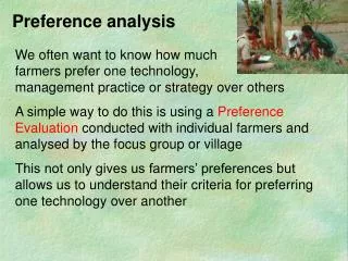
Preference Analysis. Joachim Giesen and Eva Schuberth May 24, 2006. Outline . Motivation Approximate sorting Lower bound Upper bound Aggregation Algorithm Experimental results Conclusion. Motivation. Find preference structure of consumer w.r.t. a set of products

E N D
Preference Analysis Joachim Giesen and Eva Schuberth May 24, 2006
Outline • Motivation • Approximate sorting • Lower bound • Upper bound • Aggregation • Algorithm • Experimental results • Conclusion
Motivation • Find preference structure of consumer w.r.t. a set of products • Common: assign value function to products • Value function determines a ranking of products • Elicitation: pairwise comparisons • Problem: deriving metric value function from non-metric information We restrict ourselves to finding ranking
Motivation • Efficiency measure: number of comparisons Find for every respondent a ranking individually • Comparison based sorting algorithm • Lower Bound: comparisons As set of products can be large this is too much
Motivation Possible solutions: • Approximation • Aggregation • Modeling and distribution assumptions
Approximation(joint work with J. Giesen and M. Stojaković) • Lower bound (proof) • Algorithm
Approximation • Consumer’s true ranking of n products corresponds to:Identity increasing permutation id on {1, .., n} • Wanted:Approximation of ranking corresponds to: s.t. small
Metric on Sn • Needed: metric on • Meaningful in the market research context • Spearman’s footrule metric D: • Note:
We show: To approximate ranking within expected distance at leastcomparisons necessary comparisons always sufficient
Lower bound • : randomized approximate sorting algorithm A • , If for every input permutation the expected distance of the output to id is at most r, then A performs at leastcomparisons in the worst case.
Assume less than comparisons for every input. • Fix deterministic algorithm.Then for at least permutations: output at distance more than 2r. • Expected distance of larger than r. • There is a , s.t. expected distance of larger than r.Contradiction. Lower bound: Proof Follows Yao’s Minimax Principle
Lower bound: Lemma For r>0 : ball centered at with radius r r id Lemma:
If then # sequences of n non-negative integers whose sum is at most r: Lower bound: Proof of Lemma uniquely determined by the sequence For sequence of non-negative integers : at most 2n permutations satisfy
Lower bound: deterministic case Now to show: For fixed, the number of input permutations which have output at distance more than 2r to id is more than
Lower bound: deterministic case k comparisons 2k classes of same outcome
Lower bound: deterministic case k comparisons 2k classes of same outcome
Lower bound: deterministic case For in the same class: For in the same class:
Lower bound: deterministic case For in the same class:
Lower bound: deterministic case At most 2k input permutations have same output
Lower bound: deterministic case At most input permutations with output in
Lower bound: deterministic case At least input permutations with output outside
Upper Bound Algorithm (suggested by Chazelle) approximates any ranking within distance with less than comparisons.
Algorithm • Partitioning of elements into equal sized bins • Elements within bin smaller than any element in subsequent bin. • No ordering of elements within a bin • Output: permutation consistent with sequence of bins
Algorithm Round 0 1 2
Running Time • Median search and partitioning of n elements: less than 6n comparisons (algorithm by Blum et al) • m rounds less than 6nm comparisons Distance Set Analysis of algorithm m rounds 2mbins Output : ranking consistent with ordering of bins
Algorithm: Theorem Any ranking consistent with bins computed in rounds, i.e. with less thancomparisons has distance at most
Approximation: Summary • For sufficiently large error: less comparisons than for exact sorting:error , const: comparisonserror : comparisons • For real applications: still too much • Individual elicitation of value function not possible • Second approach: Aggregation
Aggregation(joint work with J. Giesen and D. Mitsche) Motivation: • We think that population splits into preference/ customer types • Respondents answer according to their type (but deviation possible) • Instead of • Individual preference analysis or • aggregation over the population aggregate within customer types
Aggregation Idea: • Ask only a constant number of questions (pairwise comparisons) • Ask many respondents • Cluster the respondents according to answers into types • Aggregate information within a cluster to get type rankings Philosophy: First segment then aggregate
Algorithm The algorithm works in 3 phases: • Estimate the number k of customer types • Segment the respondents into the k customer types • Compute a ranking for each customer type
Algorithm Every respondent performs pairwise comparisons. Basic data structure: matrix A = [aij] Entry aij in {-1,1,0}, refers to respondent i and the j-th product pair (x,y) if respondent i prefers y over x if respondent i prefers x over y if respondent i has not compared x and y
Algorithm Define B = AAT Then Bij = number of product pairs on which respondent i and j agree minus number of pairs on which they disagree (not counting 0’s).
Algorithm: phase 1 Phase 1: Estimation of number k of customer types • Use matrix B • Analyze spectrum of B • We expect: k largest eigenvalues of B to be substantially larger than the other eigenvalues Search for gap in the eigenvalues
Algorithm: phase 2 Phase 2: Cluster respondents into customer types • Use again matrix B • Compute projector P onto the space spanned by the eigenvectors to the k largest eigenvalues of B • Every respondent corresponds to a column of P • Cluster columns of P
Algorithm: phase 2 • Intuition for using projector – example on graphs:
Algorithm: phase 2 Ad =
Algorithm: phase 2 P’ =
Algorithm: phase 2 Embedding of the columns of P
Algorithm: phase 3 Phase 3: Compute the ranking for each type • For each type t compute characteristic vector ct: • For each type t compute ATctif entry for product pair (x,y) is if respondent i belongs to that type otherwise positive: x preferred over y by t negative: y preferred over x by t zero : type t is indifferent
Experimental study On real world data • 21 data sets from Sawtooth Software, Inc. (Conjoint data sets) Questions: • Do real populations decompose into different customer types • Comparison of our algorithm to Sawtooth’s algorithm
Conjoint structures Attributes: Sets A1, .. An, |Ai|=mi An element of Ai is called level of the i-th attribute A product is an element of A1x …x An Example: Car • Number of seats = {5, 7} • Cargo area = {small, medium, large} • Horsepower = {240hp, 185hp} • Price = {$29000, $33000, $37000} • … In practical conjoint studies:
Quality measures Difficulty: we do not know the real type rankings • We cannot directly measure quality of result • Other quality measures: • Number of inverted pairs :average number of inversions in the partial rankings of respondents in type i with respect to the j-th type ranking • Deviation probability • Hit Rate (Leave one out experiments)
# respondents = 270Size of study: 8 x 3 x 4 = 96# questions = 20 Study 1 Largest eigenvalues of matrix B
# respondents = 270Size of study: 8 x 3 x 4 = 96# questions = 20 Study 1 • two types • Size of clusters: 179 – 91 Number of inversions and deviation probability
# respondents = 270Size of study: 8 x 3 x 4 = 96# questions = 20 Study 1 Hitrates: • Sawtooth: ? • Our algorithm: 69%
# respondents = 539Size of study: 4 x 3 x 3 x 5 = 180# questions = 30 Study 2 Largest eigenvalues of matrix B
# respondents = 539Size of study: 4 x 3 x 3 x 5 = 180# questions = 30 Study 2 • four types • Size of clusters: 81 – 119 – 130 – 209 Number of inversions and deviation probability
# respondents = 539Size of study: 4 x 3 x 3 x 5 = 180# questions = 30 Study 2 Hitrates: • Sawtooth: 87% • Our algorithm: 65%
# respondents = 1184Size of study: 9 x 6 x 5 = 270# questions = 48 Study 3 Size of clusters: 6 – 3 – 1164 – 8 – 3 Size of clusters: 3 – 1175 – 6 1-p = 12% Largest eigenvalues of matrix B


![Preference Elicitation [Conjoint Analysis]](https://cdn2.slideserve.com/5322185/preference-elicitation-conjoint-analysis-dt.jpg)