Point Operations

1. Point Operations

2. General Image Operations • Three type of image operations • Point operations • Geometric operations • Spatial operations

3. Point Operations

4. Point Operations • Operation depends on Pixel's value. • Context free (memory-less). • Operation can be performed on the Histogram. • Example:

5. Geometric Operations

6. Geometric Operations • Operation depend on pixel's coordinates. • Context free. • Independent of pixels value. • Example:

7. Spatial Operations

8. Spatial Operations • Operation depends on Pixel's value and coordinates. • Context dependant. • Spatial v.s. Frequency domain. • Example:

9. Point Operations • A point operation can be defined as a mapping function: where v stands for gray values. • M(v) takes any value v in the source image into vnewin the destination image. • Simplest case - Linear Mapping: M(v) q’ p’ v p q

10. If it is required to map the full gray-level range (256 values) to its full range while keeping the gray-level order - a non-decreasing monotonic mapping functionis needed: M(v) 255 stretching v 255 contraction

11. Contrast Enhancement • If most of the gray-levels in the image are in [u1 u2], the following mapping increases the image contrast. • The values u1 and u2 can be found by using the image’s accumulated histogram. M(v) 255 v u1 u2 255

12. The Negative Mapping M(v) 255 v 255

13. Point Operations and the Histogram Given a point operation: A Ca Ha M(v) M-1(v) B Cb Hb

14. Point Operations and the Histogram Given a point operation: M(va) takes any value va in image A and maps it into vb in image B. Requirement: the mapping M is a monotonic increasing function (M-1 exists). In this case, the area under Ha between 0 and va is equal to the area under Hb between 0 and vb

15. The area under Ha between 0 and va is equal to the area under Hb between 0 and vb=M(va) v M(v) vb v va Hb Ha v

16. The value of Ca at va is equal to the value of Cb at vb. v M(v) vb v va Cb Ca v

17. Q: Is it possible to obtain Hb directly from Ha and M(v)? A Ca Ha ? M(v) M-1(v) B Cb Hb

18. v M(v) vb v va Cb Ca v A: Since M(v) is monotonic, Ca(va)=Cb(vb) therefore:

19. The histogram of image B can be calculated: A Ca Ha M(v) M(v) M-1(v) B Hb Cb

20. Q: Is it possible to obtain M(v) directly from Ha and Hb ? A Ca Ha ? M(v) B Hb Cb

21. v M(v) vb v va Cb Ca v A: Since Cb is monotonic and Cb(vb)=Ca(va) Alternatively M(va)=vb if Ca(va)=Cb(vb)

22. Calculating M(v) from Ca and Cb: M(v) vb v Cb Ca v va

23. Calculating M(v) from Ca and Cb: 2-pointer Algorithm M(v) v Cb Ca v Is this always possible?

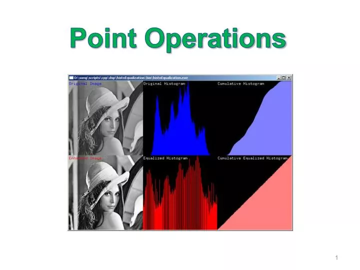
24. Histogram Equalization • Visual discrimination between objects depends on the their gray-level separation. • How can we improve discrimination after image has been acquired? Hard to discriminate Doesn’t help This is better What about this?

25. Histogram Equalization • For a better visual discrimination of an image we would like to re-assign gray-levels so that gray-level resource will be optimally assigned. • Our goal: finding a gray-level transformation M(v) such that: • The histogram Hb is as flat as possible. • The order of gray-levels is maintained. • The histogram bars are not fragmented.

26. Histogram Equalization: Algorithm • Define: • Assign: A Ha M(v) ? Ca Hb Cb

27. Hist. Eq.: The two pointers algorithm old 0 1 2 3 4 5 6 7 8 9 10 11 0 0 0 1 1 1 3 5 8 9 9 11 new

28. 30 25 30 20 (30) 25 15 (22) (21) (20) 20 10 15 5 10 0 0 1 2 3 4 5 6 7 8 9 10 11 (5) (4) (4) (4) 5 (3) (3) (3) (1) 0 0 1 2 3 4 5 6 7 8 9 10 11 Hist. Eq.: The two pointers algorithm Original Goal 30 Result 25 old 0 1 2 3 4 5 6 7 8 9 10 11 0 0 0 1 1 1 3 5 8 9 9 11 20 new 15 10 5 0 0 1 2 3 4 5 6 7 8 9 10 11

29. Hist. Eq.: Example 1 Original Equalized

30. Hist. Eq.: Example 2 Original Equalized

31. Hist. Eq.: Example 3

32. Adaptive Histogram Equalization From B. Girod, IP

33. Histogram matching • Transforms an image A so that its histogram will match that of another image B. • Usage: before comparing two images of the same scene (change detection) acquired under different lighting conditions or different camera parameters. source target mapped source

34. However, in cases where corresponding colors between images are not “consistent” this mapping may fail: from: S. Kagarlitsky: M.Sc. thesis 2010.

35. Surprising usage: Texture Synthesis (Heeger & Bergen 1995). • Start with a random image. • Step1: multi-resolution decomposition • Step2: histogram matching for each resolution • Iterate synthesis

36. More results: (Heeger & Bergen 1995):

37. Discussion: • Histogram matching produces the optimal monotonic mapping so that the resulting histogram will be as close as possible to the target histogram. • This does not necessarily imply similar images.

38. Example: Original Destination hist. match

39. Pattern Matching by Tone Mapping (MTM) (ICCV 2011) Find the BEST tone mapping between Pattern and Window Pattern Window

40. Pattern Matching by Tone Mapping (MTM) (ICCV 2011) Use the Slice Transform (SLT) to represent image as a linear sum of “slice” signals: = Image xA

41. Pattern Slices • We define a pattern slice

42. Pattern Slices 1 0 • We define a pattern slice

43. Pattern Slices * * * * * * = + 1 0 M(v) 255 v 255

44. Linear Combination of Image Slices 5 bins were used α = [0, 51, 102, 153, 204, 256] Slices are shown inverted (1 = white, 0 = black) 44

45. Pattern Slices M(v) 255 v 255

46. Example: Original Destination results SLT Hist. match

47. Point Operation on Two+ Images

48. Noise reduction by Averaging http://www.cambridgeincolour.com/tutorials

49. High Dynamic Range Images Different Exposures Combined Image Malik 1997

50. Image Subtraction Mask Image New Image Contrast Enhanced Image Difference Image http://www.isi.uu.nl/Research/Gallery/DSA/