Download

1 / 23
230 likes | 422 Views
Chi SquareTest. The statistical test used to test the null hypothesis that proportion equal or equivalently, that factors or characteristics are independent or not associated.

E N D
The statistical test used to test the null hypothesis that proportion equal or equivalently, that factors or characteristics are independent or not associated. It is used to analyze data that are presented in categories. The test applies only to discreet data, counted rather that are presented in categories. In this test, the expected frequencies and actual or obtained frequencies are compared.
The logic of the chi-square test follows: • The total number of observations in each column (treatment or control) and the total number of observations in each row (positive or negative) are considered to be given or fixed.(These column and row totals are also called marginal frequencies.) • If we assume that columns and rows are independent, we can calculate the number of observations expected to occur by chance-the expected frequencies. We find the expected frequencies by multiplying the column total by the row total and dividing by the grand total. • Expected frequency= Row Total x Column Total • Grand Total
The chi-square test compares the observed frequency in each cell with expected frequency. • If no relationship exist between the column and row variables the observed frequencies will be very close to expected frequencies; they will differ only in small amounts. In this instance, the value of chi-square statistics will be small. On the other hand, if a relationship (or dependency) does occur, the observed frequencies will vary quite a bit from the expected frequencies, and the value of the chi-square statistic will be large. • X2 (df)= ∑ (Observed frequency- Expected frequency)2 • Expected frequency • .
The Chi-square distribution: The chi-square distribution X2 (lower case Greek letter chi, pronounced like “ki” in kite, the t distribution, has degrees of freedom. In the chi-square test for independence, the number of degrees of freedom is equal to the number of rows minus 1 times the number of column minus 1 or df= (r-1)(c-1), where r is the and c the number of columns
The Chi-square goodness of fit test is used to test whether the distribution of a set of data follows a particular pattern. For example, the goodness-of-fit Chi-square may be used to test whether a set of values follow the normal distribution or whether the proportions of Democrats, Republicans, and other parties are equal to a certain set of values, say 0.4, 0.4, and 0.2.
Example: The researcher of Human Resource Department listed five items and asked each teacher to mark the one most important to her or him. The item and corresponding percentage of favorable responses are shown in Table 1.1. The HRD researcher would like to determine if the distribution of response now fits last years' distribution or if it is different.
Table 2.1 Distribution of Teachers’ Present Response on the Items Perceived Important to Them Last Year.
Problem: Is the present distribution of responses the same as last year’s? Variable: The teachers’ response on the listed items. Instrument: Survey form Null hypothesis: The present distribution of response is the same as last years’ Alternative hypothesis; The present distribution of response is different. Critical value: Referring to the critical values of chi square, at 0.05 level of significance and 4degrees of freedom, critical value is 9.49.
Since the computed value of 2.83 is less than the tabular value of 9.49, hence the null hypothesis is accepted. Therefore, at 5 percent significance level and 4 degrees of freedom, the present distribution of response is the same as last year’s. Chi –square Guidelines When testing for “goodness of fit’ at least two categories must be used to have at least 1 degree of freedom statistic. The general rule in setting up the chi-square is to have as many as possible categories for the test will then more sensitive. The limitations are no more than 20 percent of cells have an expected than the value of 5.0, and no cell has an expected frequency smaller than 1.0. If too many small expected frequencies exist, the categories should be combined, unless such combinations are not possible. If categories are combined to the point where there are only two categories and still an expected frequency of less than 5.0 exists, X2 should not be used. Instead, the binomial test may be used to treat the data.
The Chi-square test for independencein a contingency table is the most common Chi-square test. Here individuals (people, animals, or things) are classified by two (nominal or ordinal) classification variables into a two-way, contingency table. This table contains the counts of the number of individuals in each combination of the row categories and column categories. The Chi-square test determines if there is dependence (association) between the two classification variables. Hence, many surveys are analyzed with Chi-square tests.
Example: The director of the Personnel Office was interested in knowing whether the voluntary absence behavior of the school’s employees was independent of marital status. The employee files contained data on marital status with married, separated, widower, and single, and on voluntary absence behavior with categories of often absent, seldom absent, and never absent. The table gives the result for a random sample of 500 the number of employees in each cell of a two way contingency table. Test the hypothesis that voluntary absence behavior is independent of the marital status for this school. Use the α= 0.05. .
Table 2.2 Marital Status . Problem: Is the voluntary absence behavior of the school’s employees independent of their marital status? Variables: The independent variable is the employees’ marital status and the dependent variable is the employees’ voluntary absence behavior. Instrument: Employee files Null hypothesis: The voluntary absence behavior and marital status of the employees are independent. Alternative hypothesis: The voluntary absence behavior and marital status of the employees are dependent. Critical value: df= (r-1)(c-1)= (3-1)(4-1)=6 The critical value at 5 percent significance level and 6 degree of freedom is 12.59.
Table 2.3 The Employees’ Voluntary Absence Behavior and Marital Status : Since the computed value of 10.89 is less than tabular value of 12.59 at 5 percent significance level and 6 degree of freedom, accept the null hypothesis. Hence, the voluntary absence behavior and marital status of the school’s employees are independent. .
Fisher’s exact test or Fisher-Irwin Exact Test It is not appropriate for a situation in which the sample size is small, yielding small expected frequencies. There should be no expected frequencies less than 1, and not more 20% of the expected frequencies are to be less than 5. For a situation with a small sample size, we should consider using the Fisher’s Exact Test, which computes directly the probability of observing a particular set of frequencies in 2x2 tables. The formula is Fisher’s exact test P= (a+b)!(c+d)!(a+c)!(b+d)! a!b!c!d!n! where a, b, c, and d= the frequencies of 2x2table n=sample size Shortcut formula for chi-square for 2x2 tables: X2=_____n(ad-bc)2____ (a+c)(b+d)(a+b)(c+d)
Example: Consider the following 2x2 table showing the rating of successful or unsuccessful on a job and pass or fail on a ability test: Computation: P=5!4!4!5!__ = 5!4!(5∙4∙3!) = 5!4!(5∙4) = 4∙3∙2∙1(20) 9!4!1!1!3! 9!3! 9∙8∙7∙6∙5! 9∙8∙7∙6 P= 20 =0.159 126
However, to compute the P value, it is still needed to find the probability of obtaining this or a more extreme result while keeping the marginal totals in the table fixed. To do this, reduced by 1 the smallest frequency that is greater than zero while holding the marginal totals constant. Hence, the table will be: The probability of obtaining this set of frequencies is P =5!4!4!5!__ = 5!4! 9!5!0!0!4! 9! = 5!4∙3∙2∙1 9∙8∙7∙6∙5! P= 0.008
Thus the probability of observing this particular frequency of getting successful in a job or a more extreme frequency is 0.159 + 0.008= 0.167. This P value is for one-tailed test. An estimate of a P value for a two-tailed test is obtained by multiplying the value by 2; 2x 0.167= 0.334. Based on this value, the null hypothesis that there is no difference in the success of job with or without passing the ability test cannot be rejected.
Yates’ Correction for Continuity The statistic on which we base our decision has a distribution that is only approximated by the chi-square distribution. The computed X2 values depend on the cell frequencies and consequently are discrete. The continuous chi-square distribution seems to estimate the discrete sampling distribution of X2 very well, provided that the number of degrees of freedom is greater than 1. In a 2x2 contingency table, where we have only 1 degree of freedom, the Yates’ correction for continuity may be applied. It is the process of subtracting 0.5 from the numerator at each term in the chi-square statistic for 2x2 tables prior to squaring the term. X2(corrected)= ∑ (│O-E│-0.5)2 E If the expected cell frequencies are large, the corrected and uncorrected results are the same. When the expected frequencies are between 5 and 10, Yates’ correction should be applied. For expected frequencies less than 5 the Fishers’ exact test should be used.
References: Dawson and Trapp. Basic and Clinical Biostatistics 4th ed. The McGraw-Hill Companies, Inc.2004. Mangabat, Lawrence Oliver. Applied Statistics in Educational Research. http://www.en.wikipedia.org/wiki/Pearson%27s_chi-square_test. http://www.2.lv.psu.edu/jxm57/irp/chisquar.html. Submitted To: Dr. LuisitoLlido Submitted By: Cindy G. Chua Subject: Clinical Biostatistics Master of Science in Clinical Nutrition