Download
1 / 33
330 likes | 455 Views
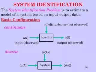
System Identification for X-dynamics. Data Analysis 4. LTP dynamics. 2 measured and controlled Degrees of Freedom within Measurement Bandwidth 3 Actuators (1 redundant) 4 Signals (2 redundant) A 2 Input-2 Output system with redundant sensing and actuation 4 Measurable transfer functions

E N D
System Identification for X-dynamics Data Analysis 4 S. Vitale
LTP dynamics S. Vitale
2 measured and controlled Degrees of Freedom within Measurement Bandwidth 3 Actuators (1 redundant) 4 Signals (2 redundant) A 2 Input-2 Output system with redundant sensing and actuation 4 Measurable transfer functions If signals are used as stimuli, separates from rest of DOF (cross-talks shows as excess noise LTP dynamics within MBW S. Vitale
Signals Dynamical variables The starting x-dynamics • In the absence of imperfections • o1 = x1 • o∆ = x2-x1 S. Vitale
Force noise Read-out noise An example, the x-dynamics S. Vitale
Control forces Force inputs An example, the x-dynamics S. Vitale
2 outputs 2 inputs An example, the x-dynamics The unmeasured variable A disappears, x1, x2, x1o1, ∆x = x2-x1 o∆ S. Vitale
An example, the x-dynamics (Frequency dependent) parameters to be measured S. Vitale
Maximum likelihood estimator S. Vitale
Maximum likelihood estimator S. Vitale
Maximum likelihood estimator S. Vitale
Signals only Maximum likelihood estimator S. Vitale
The nominal response • - open loop force on S/C • open loop difference of force on test-masses S. Vitale
The noise Channels are correlated • - open loop difference of force between test-mass 1 and S/C • open loop difference of force on test-masses S. Vitale
The noise x1 x S. Vitale
Pick matrices values that maximize Maximum likelihood estimator S. Vitale
Requires Inversion of bigN x bigN matrix Requires non linear minimization tool Maximum Likelihood S. Vitale
Good for studying the problem Allows simplified theory to be applied Allows quick estimation of Fisher Matrix and parameter resolution An alternative approach:linearisation S. Vitale
Linearization • To first order in: • # • noise S. Vitale
Imperfections 1/4 S. Vitale
Imperfections 2/4 S. Vitale
Imperfections 3/4 An elementary model for delays and roll-off S. Vitale
20 Imperfection Parameters Each parameter generates a signal Imperfections 4/4 S. Vitale
Example: Swept-sine input 0.03 mHz to 30 mHz in 104s S. Vitale
Extracting amplitudes Find h’s with no bias and minimal variance S. Vitale
Playing with a very simplified model looking for G. Very large signal S. Vitale
System identification requires Vector pre-processing (filter and linear combination) Multiple and correlated series Wiener filter/ Likelihood estimator Noise model parameterization from best measurement Dynamics pre-modeling Assessment of signals that can be uploaded ……. Conclusion S. Vitale