Download
1 / 58
590 likes | 647 Views
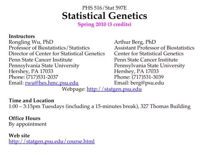
Textbook. Grading. 30% Homework (one per two weeks) 70% Research project - Class presentation (20%) - Written report (50%). Why Study Statistical Genetics?. Understand evolution and speciation. Where do we origin from?

E N D
Grading • 30% Homework (one per two weeks) • 70% Research project - Class presentation (20%) - Written report (50%)
Why Study Statistical Genetics? • Understand evolution and speciation. Where do we origin from? • Improve plant and animal breeding. How can we increase agricultural production? • Control human diseases. How can we control diseases by developing personalized medicine?
Teosinte and Maize Teosinte branched 1 (tb1) is found to affect the differentiation in branch architecture from teosinte to maize (John Doebley 2001)
Power of statistical genetics • Identify the genetic architecture of the differences in morphology between maize and teosinte • Estimate the number of genes required for the evolution of a new morphological trait from teosinte to maize: few genes of large effect or many genes of small effect? • Doebley pioneered the use of quantitative trait locus (QTL) mapping approaches to successfully identify genomic regions that are responsible for the separation of maize from its undomesticated relatives.
Doebley has cloned genes identified through QTL mapping, teosinte branched1 (tb1), which governs kernel structure and plant architecture. • Ancient Mexicans used several thousand years ago to transform the wild grass teosinte into modern maize through rounds of selective breeding for large ears of corn. • With genetic information, ‘‘I think in as few as 25 years I can move teosinte fairly far along the road to becoming maize,’’ Doebley predicts (Brownlee, 2004 PNAS vol. 101: 697–699)
Toward biomedical breakthroughs? Single Nucleotide Polymorphisms (SNPs) cancer no cancer
According to The International HapMap Consortium (2003), the statistical analysis and modeling of the links between DNA sequence variants and phenotypes will play a pivotal role in the characterization of specific genes for various diseases and, ultimately, the design of personalized medications that are optimal for individual patients. • What knowledge is needed to perform such statistical analyses? • Population genetics and quantitative genetics, and others… • The International HapMap Consortium, 2003 The International HapMap Project. Nature 426: 789-94.
Human Chromosomes Male Xy Xy FemaleXXXXXXy Daughter Son
Gene, Allele, Genotype, Phenotype Chromosomes from FatherMother Genotype Phenotype Height IQ AA 185 100 AA 182 104 Gene A, with two alleles A and a Aa 175 103 Aa 171 102 aa 155 101 aa 152 103 A question is : We cannot observe such a gene directly
Regression model for estimating the genotypic effect Phenotype = Genotype + Error yi = Σj=13xij + ei xiis the indicator for the genotype of subject i jis the mean for genotype j ei ~ N(0, 2)
Uniqueness for our genetic problem The genotypes for the trait are not observable and should be predicted from linked neutral molecular markers (M) M1 QTL M2 The genes that lead to the phenotypic variation are called Quantitative Trait Loci (QTL) M3 . . . Our task is to construct a statistical model that connects the QTL genotypes and marker genotypes through observed phenotypes Mm
(1) Mendelian genetics How does a gene transmit from a parent to its progeny (individual)? (2) Population genetics How is a gene segregating in a population (a group of individuals)? (3) Quantitative genetics How is gene segregation related with the phenotype of a character? (4) Molecular genetics What is the molecular basis of gene segregation and transmission? (5) Developmental genetics (6) Epigenetics
Mendelian Genetics Probability Population GeneticsStatistics Quantitative genetics Molecular Genetics Statistical GeneticsMathematics biology Cutting-edge research at the interface among genetics, evolution and development (Evo-Devo)
Mendel’s Laws Mendel’s first law • There is a gene with two alleles on a chromosome location (locus) • These alleles segregate during the formation of the reproductive cells, thus passing into different gametes Diploid Gene A A| a | Centromere A | a | Probability ½ ½ Gamete Gamete A pair of chromosomes
Mendel’s second law • There are two or more pairs of genes on different chromosomes • They segregate independently (partially correct) Diploid A|a|, B|b| A|, B| A|, b| a|, B| a|, b| Probability¼ ¼ ¼ ¼ Four two-gene gametes
Linkage (exception to Mendel’s second law) • There are two or more pairs of genes located on the same chromosome • They can be linked or associated (the degree of association is described by the recombination fraction) High linkage Low linkage A A B B
How the linkage occurs? – consider two genes A and B 1 2 3 4 A a A A a a A a A a A a A a B b B B b b B B b b B B b b Stage 1: A pair of chromosomes, one from the father and the other from the mother Stage 2: Each chromosome is divided into two sister chromatids Stage 3: Non-sister chromatids crossover Stage 4: Meiosis generates four gametes AB, aB, Ab and ab – Nonrecombinants (AB and ab) and Recombinants (aB and Ab)
How to measure the linkage? – based on a design Parents AABB × aabb Gamete AB ab F1 AaBb × aabb Gamete AB Ab aB ab ab Backcross AaBb Aabb aaBb aabb Observations n1 n2 n3 n4 Gamete type Non-recom/ Recom/ Recom/ Non-recom/ Parental Non-parental Non-parental Parental Define the proportion of the recombinant gametes over the total gametes as the recombination fraction (r) between two genes A and B r = (n2+n3)/(n1+n2+n3+n4)
Several concepts Genotype and Phenotype • Locus (loci), chromosomal location of a gene • Allele (A, a), a copy of gene • Dominant allele, one allele whose expression inhibits the expression of its alternative allele • Recessive allele (relative to dominant allele) • Dominant gene (AA and Aa are not distinguishable, denoted by A_) • Codominant gene (AA, Aa and aa are mutually distinguishable) • Genotype (AA, Aa or aa) • Homozygote (AA or aa) • Heterozygote (Aa) • Phenotype: trait value
Chromosome and Meiosis • Chromosome: Rod-shaped structure made of DNA • Diploid (2n): An organism or cell having two sets of chromosomes or twice the haploid number • Haploid (n): An organism or cell having only one complete set of chromosomes • Gamete: Reproductive cells involved in fertilization. The ovum is the female gamete; the spermatozoon is the male gamete. • Meiosis: A process for cell division from diploid to haploid (2n n) (two biological advantages: maintaining chromosome number unchanged and crossing over between different genes) • Crossover: The interchange of sections between pairing homologous chromosomes during meiosis • Recombination, recombinant, recombination fraction (rate, frequency): The natural formation in offspring of genetic combinations not present in parents, by the processes of crossing over or independent assortment.
Molecular markers • Genetic markers are DNA sequence polymorphisms that show Mendelian inheritance • Marker types - Restriction fragment length polymorphism (RFLP) - Amplified fragment length polymorphism (AFLP) - Simple sequence repeat (SSR) - Single nucleotide polymorphism (SNP)
Summary: Mendel’s Laws Mendel’s first law • There is a gene with two alleles on a chromosome location (locus) • These alleles segregate during the formation of the reproductive cells, thus passing into different gametes Mendel’s second law • There are two or more pairs of genes on different chromosomes • They segregate independently (partially correct) Linkage (exception to Mendel’s second law) • There are two or more pairs of genes located on the same chromosome • They can be linked or associated (the degree of association is described by the recombination fraction)
Testing Mendelian segregation Consider marker A with two alleles A and a Backcross F2 Aa aa AA Aa aa Observation n1 n0 n2 n1 n0 Expected frequency ½ ½ ¼ ½ ¼ Expected number n/2 n/2 n/4 n/2 n/4 The x2 test statistic is calculated by x2 = (obs – exp)2 /exp = (n1-n/2)2/(n/2) + (n0-n/2)2/(n/2) =(n1-n0)2/n ~x2df=1, for BC, (n2-n/4)2/(n/4)+(n1-n/2)2/(n/2)+(n0-n/4)2/(n/4)~x2df=2, for F2
Examples Backcross F2 Aa aa AA Aa aa Observation 44 59 43 86 42 Expected frequency ½ ½ ¼ ½ ¼ Expected number 51.5 51.5 42.75 85.5 42.75 The x2 test statistic is calculated by x2 = (obs – exp)2 /exp = (44-59)2/103 = 2.184 < x2df=1 = 3.841, for BC, (43-42.75)2/42.75+(86-85.5)2/85.5+(42-42.75)2/42.75=0.018 < x2df=2 =5.991, for F2 The marker under study does not deviate from Mendelian segregation in both the BC and F2.
Linkage analysis Backcross Parents AABB x aabb ABab F1 AaBb x aabb AB Ab aB abab BC AaBb Aabb aaBb aabb Obs n11 n10 n01 n00 n = nij Freq ½(1-r) ½r ½r ½(1-r) r is the recombination fraction between two markers A and B. The maximum likelihood estimate (MLE) of r is r^ = (n10+n01)/n. r has interval [0,0.5]: r=0 complete linkage, r=0.5, no linkage
Proof of r^ = (n10+n01)/n The likelihood function of r given the observations: L(r|nij) = n!/(n11!n10!n01!n00!) [½(1-r)]n11[½r]n10[½r]n01[½(1-r)]n00 = n!/(n11!n10!n01!n00!) [½(1-r)]n11+n00[½r]n10+n01 log L(r|nij) = C+(n11+n00)log[½(1-r)] +(n10+n01)log[½r] = C + (n11+n00)log(1-r) + (n10+n01)log r + nlog(½) Let the score logL(r|nij)/r = (n11+n00)[-1/(1-r)] +(n10+n01)(1/r) = 0, we have (n11+n00)[1/(1-r)]=(n10+n01)(1/r) r^ = (n10+n01)/n
Testing for linkage BC AaBb aabb Aabb aaBb Obs n11 n00 n10 n01n=nij Freq ½(1-r) ½(1-r) ½r ½r Gamete type nNR= n11+n00 nR= n10+n01 Freq with no linkage ½ ½ Exp ½n ½n 2 = (obs – exp)2/exp = (nNR - nR)2/n ~ 2df=1 Example AaBb aabb Aabb aaBb 49 47 3 4 nNR= 49+47=96 nR= 3 + 4 = 7 n=96+7=103 2 = (obs – exp)2/exp = (96-7)2/103 = 76.903 > 2df=1 = 3.841 These two markers are statistically linked. r^ = 7/103 = 0.068
Linkage analysis in the F2 BB Bb bb AA Obs n22 n21 n20 Freq ¼(1-r)2½r(1-r)¼r2 Aa Obs n12 n11 n10 Freq ½r(1-r)½(1-r)2+½r2½r(1-r) aa Obs n02 n01 n00 Freq ¼r2½r(1-r)¼(1-r)2 Likelihood function L(r|nij) = n!/(n22!...n00!) [¼(1-r)2]n22+n00[¼r2]n20+n02[½r(1-r)]n21+n12+n10+n01 [½(1-r)2+½r2]n11 Let the score = 0 so as to obtain the MLE of r, but this will be difficult because AaBb contains a mix of two genotype formation types (in the dominator we will have ½(1-r)2+½r2).
I will propose a shortcut EM algorithm for obtain the MLE of r BB Bb bb AA Obs n22 n21 n20 Freq ¼(1-r)2½r(1-r)¼r2 Recombinant 0 1 2 Aa Obs n12 n11 n10 Freq ½r(1-r)½(1-r)2+½r2½r(1-r) Recombinant 1 2r2/[(1-r)2+r2] 1 aa Obs n02 n01 n00 Freq ¼r2½r(1-r)¼(1-r)2 Recombinant 2 1 0
Based on the distribution of the recombinants (i.e., r), we have r = 1/(2n)[2(n20+n02)+(n21+n12+n10+n01)+2r2/[(1-r)2+r2]n11 (1) = 1/(2n)(2n2R + n1R + 2n11) where n2R = n20+n02, n1R = n21+n12+n10+n01, n0R = n22+n00. The EM algorithm is formulated as follows E step: Calculate 2 = 2r2/[(1-r)2+r2] (expected the number of recombination events for the double heterozygote AaBb) M step: Calculate r^ by substituting the calculated from the E step into Equation 1 Repeat the E and M step until the estimate of r is stable
Example BB Bb bb AA n22=20 n21 =17 n20=3 Aa n12 =20n11 =49n10 =19 aa n02=3n01 =21 n00=19 Calculating steps: 1. Give an initiate value for r, r(1) =0.1, 2. Calculate (1)=(r(1))2/[(1- r(1))2+(r(1))2] = 0.12/[(1-0.1)2+0.12] = x; 3. Estimate r using Equation 1, r(2) = y; • Repeat steps 2 and 3 until the estimate of r is stable (converges). The MLE of r = 0.31. How to determine that r has converged? |r(t+1) – r(r)| < a very small number, e.g., e-8
Testing the linkage in the F2 BB Bb bb AA Obs n22=20 n21 =17 n20=3 Exp with no linkage 1/16n 1/8n 1/16n Aa Obs n12 =20n11 =49n10 =19 Exp with no linkage 1/8n ¼n 1/8n aa Obs n02=3n01 =21 n00=19 Exp with no linkage 1/16n 1/8n 1/16n n = nij = 191 2 = (obs – exp)2/exp ~ 2df=1 = (20-1/16×191)/(1/16×191) + … = a > 2df=1=3.381 Therefore, the two markers are significantly linked.
Log-likelihood ratio test statistic Two alternative hypotheses H0: r = 0.5 vs. H1: r 0.5 Likelihood value under H1 L1(r|nij) = n!/(n22!...n00!) [¼(1-r)2]n22+n00[¼r2]n20+n02[½r(1-r)]n21+n12+n10+n01[½(1-r)2+½r2]n11 Likelihood value under H0 L0(r=0.5|nij) = n!/(n22!...n00!) [¼(1-0.5)2]n22+n00[¼0.52]n20+n02[½0.5(1-0.5)]n21+n12+n10+n01[½(1-0.5)2+½0.52]n11 LOD = log10[L1(r|nij)/L0(r=0.5|nij)] = {(n22+n00)2[log10(1-r)-log10(1-0.5)+…} = 6.08 > critical LOD=3
Three-point analysis • Determine a most likely gene order; • Make full use of information about gene segregation and recombination Consider three genes A, B and C. Three possible orders A-B-C, A-C-B, or B-A-C
AaBbCc produces 8 types of gametes (haplotypes) which are classified into four groups Recombinant # between Observation Frequency A and BB and C ABC and abc 0 0 n00=nABC+nabc g00 ABc and abC 0 1 n01=nAbc+nabC g01 aBC and Abc 1 0 n10=naBC+nAbc g10 AbC and aBc 1 1 n11=nAbC+naBc g11 Note that the first subscript of n or g denotes the number of recombinant between A and B, whereas the second subscript of n or g denotes the number of recombinant between B and C (assuming order A-B-C)
Matrix notation Markers B and C Markers A and B Recombinant Non-recombinant Total Recombinant n11 n10 Non-recombinant n01 n00 Total n Recombinant g11 g10 rAB Non-recombinant g01 g00 1-rAB Total rBC 1-rBC 1 What is the recombination fraction between A and C? rAC = g01 + g10 Thus, we have rAB = g11 + g10 rBC = g11 + g01 rAC = g01 + g10
The data log-likelihood (complete data, it is easy to derive the MLEs of gij’s) log L(g00, g01, g10, g11| n00, n01, n10, n11, n) = log n! – (log n00! + log n01! + log n10! + log n11!) + n00 log g00 + n01 log g01 + n10 log g10+ n11 log g11 The MLE of gij is: Based on the invariance property of the MLE, we obtain the MLE of rAB, rAC and rBC. A relation: 0 g11 = ½(rAB + rBC - rAC) rAC rAB + rBC 0 g10 = ½(rAB - rBC + rAC) rBC rAB + rAC 0 g01 = ½(-rAB + rBC + rAC) rAB rAC + rBC
Advantages of three-point (and generally multi-point) analysis • Determine the gene order, • Increase the estimation precision of the recombination fractions (for partially informative markers).
Real-life example – AoC/oBo ABC/ooo Eight groups of offspring genotypes A_B_C_ A_B_cc A_bbC_ A_bbcc aaB_C_ aaV_cc aabbC_ aabbcc Obs. 28 4 12 3 1 8 2 2 Order A - B - C Two-point analysis 0.380.386 0.390.418 0.180.056 Three-point analysis 0.200.130 0.200.130 0.200.059
Multilocus likelihood – determination of a most likely gene order • Consider three markers A, B, C, with no particular order assumed. • A triply heterozygous F1 ABC/abc backcrossed to a pure parent abc/abc Genotype ABC or abc ABc or abC Abc or aBC AbC or aBc Obs. n00 n01 n10 n11 Frequency under Order A-B-C (1-rAB)(1- rBC) (1-rAB) rBC rAB(1- rBC) rAB rBC Order A-C-B (1-rAC)(1- rBC) rAC rBC rAC(1-rBC)(1-rAC)rBC Order B-A-C (1-rAB)(1- rAC) (1-rAB) rAC rABrAC rAB(1-rAC) rAB = the recombination fraction between A and B rBC = the recombination fraction between B and C rAC = the recombination fraction between A and C
It is obvious that rAB = (n10 + n11)/n rBC = (n01 + n11)/n rAC = (n01 + n10)/n What order is the mostly likely? LABC (1-rAB)n00+n01 (1-rBC)n00+n10 (rAB)n10+n11 (rBC)n01+n11 LACB (1-rAC)n00+n11 (1-rBC)n00+n10 (rAC)n01+n10 (rBC)n01+n11 LBAC (1-rAB)n00+n01 (1-rAC)n00+n11 (rAB)n10+n11 (rAC)n01+n10 According to the maximum likelihood principle, the linkage order that gives the maximum likelihood for a data set is the best linkage order supported by the data. This can be extended to include many markers for searching for the best linkage order.