Download

1 / 73
740 likes | 873 Views
Techniques Based on Recursion. Lecturer: Jing Liu Email: neouma@mail.xidian.edu.cn Homepage: http://see.xidian.edu.cn/faculty/liujing Xidian Homepage: http://web.xidian.edu.cn/liujing. What ’ s Recursion?.

E N D
Techniques Based on Recursion Lecturer: Jing Liu Email: neouma@mail.xidian.edu.cn Homepage: http://see.xidian.edu.cn/faculty/liujing Xidian Homepage: http://web.xidian.edu.cn/liujing
What’s Recursion? • Recursion is the process of dividing the problem into one or more subproblems, which are identical in structure to the original problem and then combining the solutions to these subproblems to obtain the solution to the original problem.
What’s Recursion? • There are three special cases of the recursion technique: • Induction: the idea of induction in mathematical proofs is carried over to the design of efficient algorithms • Nonoverlapping subproblems: divide and conquer • Overlapping subproblems: dynamic programming, trading space for time
Induction Given a problem with parameter n, designing an algorithm by induction is based on the fact that if we know how to solve the problem when presented with a parameter less than n, called the induction hypothesis, then our task reduces to extending that solution to include those instances with parameter n.
Radix Sort • Let L={a1, a2, …, an} be a list of n numbers each consisting of exactly k digits. That is, each number is of the form dkdk-1…d1, where each di is a digit between 0 and 9. • In this problem, instead of applying induction on n, the number of objects, we use induction on k, the size of each integer.
Radix Sort • If the numbers are first distributed into the lists by their least significant digit, then a very efficient algorithm results. • Suppose that the numbers are sorted lexicographically according to their least k-1 digits, i.e., digits dk-1, dk-2, …, d1. • After sorting them on their kth digits, they will eventually be sorted.
Radix Sort • First, distribute the numbers into 10 lists L0, L1, …, L9 according to digit d1 so that those numbers with d1=0 constitute list L0, those with d1=1 constitute list L1 and so on. • Next, the lists are coalesced in the order L0, L1, …, L9. • Then, they are distributed into 10 lists according to digit d2, coalesced in order, and so on. • After distributing them according to dk and collecting them in order, all numbers will be sorted.
Radix Sort Example: Sort A nondecreasingly. A[1…5]=7467 3275 6792 9134 1239
Radix Sort • Input: A linked list of numbers L={a1, a2, …, an} and k, the number of digits. • Output: L sorted in nondecreasing order. 1. for j1 to k 2. Prepare 10 empty lists L0, L1, …, L9; 3. while L is not empty 4. anext element in L; 5. Delete a from L; 6. ijth digit in a; 7. Append a to list Li; 8. end while; 9. L L0; 10. for i 1 to 9 11. LL, Li //Append list Li to L 12. end for; 13. end for; 14. return L;
Radix Sort • What’s the performance of the algorithm Radix Sort? • Time Complexity? • Space Complexity?
Radix Sort • Time Complexity: (n) • Space Complexity: (n)
Generating Permutations • Generating all permutations of the numbers 1, 2, …, n. • Based on the assumption that if we can generate all the permutations of n-1 numbers, then we can get algorithms for generating all the permutations of n numbers.
Generating Permutations • Generate all the permutations of the numbers 2, 3, …, n and add the number 1 to the beginning of each permutation. • Generate all permutations of the numbers 1, 3, 4, …, n and add the number 2 to the beginning of each permutation. • Repeat this procedure until finally the permutations of 1, 2, …, n-1 are generated and the number n is added at the beginning of each permutation.
Input: A positive integer n; • Output: All permutations of the numbers 1, 2, …, n; • 1. for j1 to n • 2. P[j]j; • 3. end for; • 4. perm(1); • perm(m) • 1. if m=n then output P[1…n] • 2. else • 3. for jm to n • 4. interchange P[j] and P[m]; • //Add one number at the beginning of the permutation • 5. perm(m+1); • //Generate permutations for the left numbers • 6. interchange P[j] and P[m]; • 7. end for; • 8. end if;
Generating Permutations • What is the recursion process? • Write codes to implement the algorithms.
Generating Permutations • What’s the performance of the algorithm Generating Permutations? • Time Complexity? • Space Complexity?
Generating Permutations • Time Complexity: (nn!) • Space Complexity: (n)
Finding the Majority Element • Let A[1…n] be a sequence of integers. An integer a in A is called the majority if it appears more thann/2 times in A. • For example: • Sequence 1, 3, 2, 3, 3, 4, 3: 3 is the majority element since 3 appears 4 times which is more than n/2 • Sequence 1, 3, 2, 3, 3, 4: 3 is not the majority element since 3 appears three times which is equal to n/2, but not more than n/2
Finding the Majority Element • If two different elements in the original sequence are removed, then the majority in the original sequence remains the majority in the new sequence. • The above observation suggests the following procedure for finding an element that is candidate for being the majority.
Finding the Majority Element • Let x=A[1] and set a counter to 1. • Starting from A[2], scan the elements one by one increasing the counter by one if the current element is equal to x and decreasing the counter by one if the current element is not equal to x. • If all the elements have been scanned and the counter is greater than zero, then return x as the candidate. • If the counter becomes 0 when comparing x with A[j], 1<j<n, then call procedure candidate recursively on the elements A[j+1…n].
Finding the Majority Element • Why just return x as a candidate? Restart Count=1 4 4 4 1 2 3 5 Count=0 But 5 is not the majority element.
Input: An array A[1…n] of n elements; • Output: The majority element if it exists; otherwise none; • 1. xcandidate(1); • 2. count0; • 3. for j1 to n • 4. if A[j]=x then countcount+1; • 5. end for; • 6. if count>n/2 then return x; • 7. else return none; • candidate(m) • 1. jm; xA[m]; count1; • 2. while j<n and count>0 • 3. j j+1; • 4. if A[j]=x then count count+1; • 5. else count count-1; • 6. end while; • 7. if j=n then return x; • 8. else return candidate(j+1);
Divide and Conquer • A divide-and-conquer algorithm divides the problem instance into a number of subinstances (in most cases 2), recursively solves each subinsance separately, and then combines the solutions to the subinstances to obtain the solution to the original problem instance.
Divide and Conquer • Consider the problem of finding both the minimum and maximum in an array of integers A[1…n] and assume for simplicity that n is a power of 2. • Divide the input array into two halves A[1…n/2] and A[(n/2)+1…n], find the minimum and maximum in each half and return the minimum of the two minima and the maximum of the two maxima.
Divide and Conquer • Input: An array A[1…n] of n integers, where n is a power of 2; • Output: (x, y): the minimum and maximum integers in A; • 1. minmax(1, n); • minmax(low, high) • 1. if high-low=1 then • 2. if A[low]<A[high] then return (A[low], A[high]); • 3. else return(A[high], A[low]); • 4. end if; • 5. else • 6. mid(low+high)/2; • 7. (x1, y1)minmax(low, mid); • 8. (x2, y2)minmax(mid+1, high); • 9. xmin{x1, x2}; • 10. y max{y1, y2}; • 11. return(x, y); • 12. end if;
Divide and Conquer • How many comparisons does this algorithm need?
Divide and Conquer • Given an array A[1…n] of n elements, where n is a power of 2, it is possible to find both the minimum and maximum of the elements in A using only (3n/2)-2 element comparisons.
The Divide and Conquer Paradigm • The divide step: the input is partitioned into p1 parts, each of size strictly less than n. • The conquer step: performing p recursive call(s) if the problem size is greater than some predefined threshold n0. • The combine step: the solutions to the p recursive call(s) are combined to obtain the desired output.
The Divide and Conquer Paradigm • (1) If the size of the instance I is “small”, then solve the problem using a straightforward method and return the answer. Otherwise, continue to the next step; • (2) Divide the instance I into p subinstances I1, I2, …, Ip of approximately the same size; • (3) Recursively call the algorithm on each subinstance Ij, 1jp, to obtain p partial solutions; • (4) Combine the results of the p partial solutions to obtain the solution to the original instance I. Return the solution of instance I.
Selection: Finding the Median and the kth Smallest Element • The media of a sequence of n sorted numbers A[1…n] is the “middle” element. • If n is odd, then the middle element is the (n+1)/2th element in the sequence. • If n is even, then there are two middle elements occurring at positions n/2 and n/2+1. In this case, we will choose the n/2th smallest element. • Thus, in both cases, the median is the n/2th smallest element. • The kth smallest element is a general case.
Selection: Finding the Median and the kth Smallest Element • If we select an element mm among A, then A can be divided in to 3 parts:
Selection: Finding the Median and the kth Smallest Element • According to the number elements in A1, A2, A3, there are following three cases. In each case, where is the kth smallest element?
Selection: Finding the Median and the kth Smallest Element • Input: An array A[1…n] of n elements and an integer k, 1kn; • Output: The kth smallest element in A; • 1. select(A, 1, n, k);
Selection: Finding the Median and the kth Smallest Element • select(A, low, high, k) • 1. phigh-low+1; • 2. if p<44 then sort A and return (A[k]); • 3. Let q=p/5. Divide A into q groups of 5 elements each. • If 5 does not divide p, then discard the remaining elements; • 4. Sort each of the q groups individually and extract its media. • Let the set of medians be M. • 5. mmselect(M, 1, q, q/2); • 6. Partition A[low…high] into three arrays: • A1={a|a<mm}, A2={a|a=mm}, A3={a|a>mm}; • 7. case • |A1|k: return select (A1, 1, |A1|, k); • |A1|+|A2|k: return mm; • |A1|+|A2|<k: return select(A3, 1, |A3|, k-|A1|-|A2|); • 8. end case;
Selection: Finding the Median and the kth Smallest Element • What is the time complexity of this algorithm?
Selection: Finding the Median and the kth Smallest Element • The kth smallest element in a set of n elements drawn from a linearly ordered set can be found in (n) time.
Quicksort • Let A[low…high] be an array of n numbers, and x=A[low]. • We consider the problem of rearranging the elements in A so that all elements less than or equal to x precede x which in turn precedes all elements greater than x. • After permuting the element in the array, x will be A[w] for some w, lowwhigh. The action of rearrangement is also called splitting or partitioning around x, which is called the pivot or splitting element.
Quicksort • We say that an element A[j] is in its proper position or correct position if it is neither smaller than the elements in A[low…j-1] nor larger than the elements in A[j+1…high]. • After partitioning an array A using xA as a pivot, x will be in its correct position.
Quicksort • Input: An array of elements A[low…high]; • Output: (1) A with its elements rearranged, if necessary; • (2) w, the new position of the splitting element A[low]; • 1. ilow; • 2. xA[low]; • 3. for jlow+1 to high • 4. if A[j]x then • 5. ii+1; • 6. if ij then interchange A[i] and A[j]; • 7. end if; • 8. end for; • 9. interchange A[low] and A[i]; • 10.wi; • 11.return A and w;
Quicksort • The number of element comparisons performed by Algorithm SPLIT is exactly n-1. Thus, its time complexity is (n). • The only extra space used is that needed to hold its local variables. Therefore, the space complexity is (1).
Quicksort • Input: An array A[1…n] of n elements; • Output: The elements in A sorted in nondecreasing order; • 1. quicksort(A, 1, n); • quicksort(A, low, high) • 1. if low<high then • 2. SPLIT(A[low…high], w) \\w is the new position of A[low]; • 3. quicksort(A, low, w-1); • 4. quicksort(A, w+1, high); • 5. end if;
Quicksort • The average number of comparisons performed by Algorithm QUICKSORT to sort an array of n elements is (nlogn).
Dynamic Programming • An algorithm that employs the dynamic programming technique is not recursive by itself, but the underlying solution of the problem is usually stated in the form of a recursive function. • This technique resorts to evaluating the recurrence in a bottom-up manner, saving intermediate results that are used later on to compute the desired solution. • This technique applies to many combinatorial optimization problems to derive efficient algorithms.
Dynamic Programming • Fibonacci sequence: f1=1 f2=1 f3=2 f4=3 f5=5 f6=8 f7=13 …… • f(n) • 1. if (n=1) or (n=2) then return 1; • 2. else return f(n-1)+f(n-2); • This algorithm is far from being efficient, as there are many duplicate recursive calls to the procedure.
Dynamic Programming • f(n) • 1. if (n=1) or (n=2) then return 1; • 2. else • 3. { • 4. fn_1=1; • 5. fn_2=1; • 6. for i3 to n • 7. fn=fn_1+fn_2; • 8. fn_2=fn_1; • 9. fn_1=fn; • 10. end for; • 11. } • 12. Return fn; • Time: n-2 additions (n) • Space: (1)
The Longest Common Subsequence Problem • Given two strings A and B of lengths n and m, respectively, over an alphabet , determine the length of the longest subsequence that is common to both A and B. • A subsequence of A=a1a2…an is a string of the form ai1ai2…aik, where each ij is between 1 and n and 1i1<i2<…<ikn.
The Longest Common Subsequence Problem • Let A=a1a2…an and B=b1b2…bm. • Let L[i, j] denote the length of a longest common subsequence of a1a2…ai and b1b2…bj. 0in, 0jm. When i or j be 0, it means the corresponding string is empty. • Naturally, if i=0 or j=0; the L[i, j]=0
The Longest Common Subsequence Problem Suppose that both i and j are greater than 0. Then • If ai=bj, L[i, j]=L[i-1, j-1]+1 • If aibj, L[i, j]=max{L[i, j-1], L[i-1, j]} We get the following recurrence for computing the length of the longest common subsequence of A and B:
The Longest Common Subsequence Problem • We use an (n+1)(m+1) table to compute the values of L[i, j] for each pair of values of i and j, 0in, 0jm. • We only need to fill the table L[0…n, 0…m] row by row using the previous formula.
The Longest Common Subsequence Problem • Example: A=zxyxyz, B=xyyzx What is the longest common subsequence of A and B?