Download
1 / 17
190 likes | 327 Views
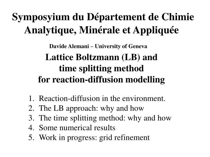
Symposyium du Département de Chimie Analytique, Minérale et Appliquée Davide Alemani – University of Geneva Lattice Boltzmann (LB) and time splitting method for reaction-diffusion modelling. Reaction-diffusion in the environment. The LB approach: why and how

E N D
Symposyium du Département de Chimie Analytique, Minérale et AppliquéeDavide Alemani – University of GenevaLattice Boltzmann (LB) andtime splitting methodfor reaction-diffusion modelling • Reaction-diffusion in the environment. • The LB approach: why and how • The time splitting method: why and how • Some numerical results • Work in progress: grid refinement
Schematic representation of various chemical species of a given element (M)
Schematic representation of the physicochemical problem under investigation Metal concentration: 10-7 mol/m3 - 10-3 mol/m3 Diffusion coefficient: 10-12 m2/s - 10-9 m2/s Kinetic rate constants: 10-6 s-1 - 109 s-1
LB approach: Why and how Macroscopic Model Mesoscopic Model (LB) M L ML
The LBGK model (1D) LBGK Evolution Equations Schematic Representation (1D) Flux Computation
Time splitting method: Why and How • Important when physical and chemical processes occur simultaneously and rate constants vary over many order of magnitudes • Enables to split a complex problem into two or more sub-problems more simply handled NS RD
A detailed example of Time Splitting (RD) coupled with LBGK approach M L ML
Flux at the electrode for a semilabile complex Labile flux: Numerical flux: Inert flux:
Comparison between RD and NS with an exact solution Red circle values are taken from: De Jong et al., JEC 1987, 234, 1
Flux at the electrode for two complexes ML(1) and ML(2) with very different time scale reaction rates M+L(1)ML(1) labile – M+L(2)ML(2) inert Labile flux: Numerical flux: Inert flux:
M+L(1)ML(1) labile – M+L(2)ML(2) inert Concentration profiles close to the electrode Strong variation close to the electrode surface
Work in progress A grid refinement approach for solving LBGK scheme Problem to solve M + L(n) ML(n)
Work in progress A grid refinement approach for solving LBGK scheme Conservation of mass and flux at the grid interface
That’s all.Thanks to comeHoping to have been clearHave a nice day