Download
1 / 17
200 likes | 397 Views
CAM(2+) Coupled to a Mixed Layer Ocean Model: Model Physics and Climate. Christophe Cassou Mike Alexander Clara Deser. CCSM Workshop Santa Fe 2004. In the code, COUP_MLM is equivalent to COUP_SOM, which allows for coupling with a Slab Ocean Model (SOM). Slab Ocean. Mixed Layer Model.

E N D
CAM(2+) Coupled to a Mixed Layer Ocean Model: Model Physics and Climate Christophe Cassou Mike Alexander Clara Deser CCSM Workshop Santa Fe 2004
In the code, COUP_MLM is equivalent to COUP_SOM, which allows for coupling with a Slab Ocean Model (SOM) Slab Ocean Mixed Layer Model Qnet Qcor Qnet Qcor Varying H Tm Fixed H Tm/Sm Tb/Sb DTm = Qnet/rcH +Qcor/rcH Accounts for vertical processes What is the COUP_MLM option? 1.1 Introduction : the model Coupling between CAM (2+) - ocean Mixed Layer Model (MLM) - the thermodynamic portion of the NCAR sea ice model (CSIM4)
MLM in more detail 1.2 Introduction : the model An individual column model with a uniform mixed layer atop a layered model that represents conditions in the pycnocline MLM model: Alexander et al (2002, J. Clim) based on Gaspar’s (1988, JPO) formulation • Model characteristics: • Same grids as the atmosphere (128 lon x 64 lat) • 36 vertical levels (from 0m to 1500m depth) with a • better resolution close to surface (10 levels for the first 50m) • Realistic bathymetry
Diffusion Qcor Qnet Qwe Solar Penetration Vertical Entrainment (We from turbulent Kinetic energy equation) Qswh Convective Adjustment CA Mixed layer Temperature change in MLM 1.3 Introduction: the model h (MLD) Tm1 Tb1
The salinity equation 1.4 Introduction: the model Below ice there is fresh water flux due to: - ice volume change - brine ejection weighted by the ice fraction
Max : +0.8 Max : +1 • SST bias tied to ice (ovals) • ice melts early Labrador Sea • Ice melt late north of Russia Max : +1.2 SST too warm in summer due to over-estimated shoaling SST biais 2.1 Validation of the climatology Departure between 80yr mean and observed (HADISST) climatology January July
Underestimates of the MLD Correct representation Over the main atm. Baroclinic zone Overestimation over theTrade winds domain and no diurnal cycle Mixed Layer Depth 2.2 Validation of the climatology 80y mean MLD for January-February-March average
Ice concentration (Northern Hemisphere) 2.3 Validation of the climatology Model (80y mean) March September Observations Realistic SI Extent but UNrealistic SI Thickness
Ice concentration (Southern Hemisphere) 2.4 Validation of the climatology Model (80y mean) March September Observations
PC1 (bars)/5yr-running mean (green line) Regressed MSLP Variability in the Indian Ocean and its links to the atmosphere 3.1 Variability EOF1 for DJF SST(contour) /Regressed precipitation (filled)
No significant auto-corr. for MSLP (white noise) + Quasi-biennal dominant peak MSLP SST SST MSLP Reddening of the SST spectrum Years Variability in the North Pacific 3.2 Variability SVD between SST (color) and MSLP (contour) FMA season
No significant auto-corr. for MSLP (white noise) + Quasi-biennal dominant peak SST MSLP SST MSLP Reddening of the SST spectrum Years Variability in the North Atlantic 3.3 Variability SVD between SST (color) and MSLP (contour) FMA season
Regressed ice frac Regressed Mixed Layer Depth Deeper Shallower More Ice Less Ice The North Atlantic Osciallation 3.4 Variability EOF1 for DJF MSLP(contour) Regressed SST(filled) White spectrum with a strong quasi-biennal peak Strongly linked to the Artic Oscillation
+0.5 +0.6 Oct (+7) Jan (+10) Persistence of SST anomalies : Monthly Autocorrelation 3.5 Variability From March (0) 60 30 May (+2)
Relationship between the deep ocean and the surface atmosphere 3.6 Variability 3D SVD between JAS Ocean Temperature [30m-400m] (color @30m) and previous FMA MSLP (contour)
Reemergence mechanism Oct (+7) Jan (+10) The Reemergence mechanism 3.7 Variability From March (0) 60 30 May (+2) +0.5 +0.6
Model has run for more than 150 years now and appears to be stable (basic climate variability structures are correctly simulated, some biais though –model and configuration) Originally MLM coupled to CAM2 plan is to support with newer versions of CAM (coupled with CAM3 in progress) Ocean can be a mix of specified SSTs and MLM (e.g. observed SSTs specified in the tropical Pacific) Useful for a wide variety of coupled model studies: between CAM-SOM CCSM (Reemergence experiments running right now) Will be used in climate@home project (See J. Hansen, MIT) Discussion