Download
1 / 105
1.11k likes | 1.44k Views
Mesoscale Modeling. Robert Rozumalski National SOO Science and Training Resource Coordinator NOAA/NWS/OCWWS/FDTB. Tour of Talk. Introduction and mesoscale primer Model Resolution Hydrostatic vs. Non-Hydrostatic Mesoscale Model Physics Mesoscale Model Boundaries Simple Model Experiments.

E N D
Mesoscale Modeling Robert Rozumalski National SOO Science and Training Resource CoordinatorNOAA/NWS/OCWWS/FDTB
Tour of Talk • Introduction and mesoscale primer • Model Resolution • Hydrostatic vs. Non-Hydrostatic • Mesoscale Model Physics • Mesoscale Model Boundaries • Simple Model Experiments
A Very Brief Mesoscale Primer • NWP is the application of the Navier-Stokes equations that have been adapted to atmospheric flow • But are mesoscale models simply NWP models applied at a smaller grid spacing? • Yes – mesoscale models are simply NWP systems that have been designed to simulate mesoscale atmospheric phenomena
A Very Brief Mesoscale Primer • Term “mesoscale” attributed to Lidga (1951) to classify phenomena that were observed on radar but not from conventional observation • Since then a number of classification schemes have been proposed (Orlanski, 1975; Fujita, 1981, etc.) • Traditional definition of mesoscale – from 2 to 2,000 km (Orlanski, 1975) • 500 km grid spacing - mesoscale model? • 2 km grid spacing - mesoscale model? • The model results differ but may still be classified as mesoscale by the above definition
A Very Brief Mesoscale Primer • An alternative mesoscale definition (Emanuel, Pielke): • The horizontal scale must be sufficiently small so that the Coriolis term is small relative to the advective and pressure gradient forces • Defines the upper bound • Definition is a function of latitude • Near equator much larger meteorological features are considered “mesoscale” than at the poles
A Very Brief Mesoscale Primer • An alternative mesoscale definition (Emanuel, Pielke): • The horizontal scale must be sufficiently large so that the hydrostatic approximation can be applied • Defines the lower bound Given the above definition of “mesoscale”: Q: If you are running non-hydrostatic dynamics are you still using a mesoscale model? Q: Is a model running at a 1 km grid spacing considered mesoscale?
Resolution and Grid Spacing Basics: A value at a model grid point represents the mean within a Dx * Dy * Dz grid cell or box
Resolution and Grid Spacing • Basics:A model forecast at a grid point does not represent an actual maximum or minimum value unless: • There is no variability within the grid cell • The grid cell is infinitesimal=> point Wind Speeds
Resolution and Grid Spacing • Basics:Grid-point models can adequately resolve features that are 4Dx (5 grid points) or greater • Basics:The 12 km NAM can resolve features on a scale of 48 km or greater
Resolution and Grid Spacing • Basics: “adequately resolve” does not mean well-resolved
Horizontal Resolution Feature A: Covers an area spanning > 5 grid points: May appear in model fieldsFeature B: Covers an area spanning 1-2 grid points: Will not appear
Vertical Resolution When deciding how to define the vertical resolution in an NWP model: • The vertical structure should be prescribed to fully resolve the critical vertical circulations in a simulation • A greater tilt to the system being simulated requires increased vertical resolution
Vertical Resolution • Most model configurations attempt to place the highest vertical resolution where it is needed most, near the earth surface • This allows the model to better resolve the transfer of heat and moisture into the boundary layer
Vertical Resolution • Similar resolution is generally not necessary in the middle troposphere (~600 to 300 mb) since vertical mixing has a longer length scale • An increase in resolution is preferable within the upper troposphere to accurately resolve the jet stream circulations
Vertical Resolution 21 Levels 31 Levels 61 Levels Model Top Model Top Model Top
Vertical Resolution 3 km simulation 15 levels 61 levels
Vertical Resolution 3 km simulation 15 levels 61 levels
Temporal Resolution • An NWP model moves (integrates) forward in time by discrete time steps using a finite difference scheme • Leap Frog - 1st order accuracy (faster) • Runge-Kutta – 3rd order accuracy (slower: ARW) • One limitation is that a trade-off exists between numerical accuracy and computational efficiency • Type of scheme used: higher order -> more accuracy -> slower • Smaller time step, more numerical accuracy, slower model runs • Larger time steps, less numerical accuracy, faster model runs
Temporal Resolution • Generally, the need for computational efficiencyoverrides that of computational accuracy; however, there is a limit: • A fundamental governing condition for the integration of time in a numerical model is the Courant, Friedrichs, and Lewy (CFL) condition • The CFL condition states that the time step between intermediate forecasts must be less than the time it takes the fastest moving wave in the model to travel one grid space (Dx)
Temporal Resolution • A violation of the CFL condition is most commonly manifested as numerical “noise” often followed by a model crash (Bummer).
Temporal Resolution 3 km simulation 18s Timestep 9s Timestep
Resolution Vs. Computational Speed • The computational cost of increasing vertical resolution is less than increasing the horizontal resolution • 2-fold increase in levels ~ 2x increase in computation time • 2-fold decrease in horizontal grid spacing ~ 8x increase in computationtime (3-fold = 27x increase!) • However, the potential benefit from a decrease in the grid spacing may be much greater than an increase in vertical levels • There is generally little value in decreasing the model timestep to increase numerical accuracy
Hydrostatic Vs. Non-Hydrostatic Examples of Processes with NH Effects Solar Radiation Fluxes Convection Solar Radiation Moisture Fluxes Turbulence Evaporation Condensation Fluxes Surface heating Surface heating
Hydrostatic Vs. Non-Hydrostatic • Until recently, running an NWP model at resolutions capable of resolving non-hydrostatic phenomena was very computationally expensive • Small scale feature => small Dx => small Dt • Additional cost in predicting vertical motion • Most users accepted the hydrostatic approximation
Hydrostatic Vs. Non-Hydrostatic • Vertical Equation of Motion • At large horizontal scales, i.e, Lx >> Lz, the gravitational term is very large compared to buoyancy • As scale becomes smaller, the buoyancy term may become more important
Hydrostatic Vs. Non-Hydrostatic • So, when do you need to go non-hydrostatic? • Traditional rational is Dx < 10 km • Some have noted that NH contribution not important until Dx ~ 1km • Depends upon the phenomenon of interest! • Explicitly resolved convection with Dx=4 km ~ NH • Outflow boundary from convection with Dx=4 km ~ NH • Sea breeze circulation with Dx=3 km ~ HY or NH • Gravity wave simulation with Dx=5 km ~HY or NH • Large scale baroclinic wave with Dx=5 km ~ HY • Flow over topography with Dx=2 km ~ Depends on topography • Cost of NH dynamics with ARW WRF ~ 5%
Hydrostatic Vs. Non-Hydrostatic 10 m/s Dx = 10 km : Hydro or NH dynamics? Probably does not make a difference since forcing is of the scale where hydrostatic dynamics dominate Dx = 1km : Hydro or NH dynamics? Lx (100 km) >> Lz (1 km) 10 km 1km 100 km Obviously not to scale
Hydrostatic Vs. Non-Hydrostatic 3 km simulation Hydrostatic Non-Hydrostatic
Hydrostatic Vs. Non-Hydrostatic 3 km simulation Hydrostatic Non-Hydrostatic
Mesoscale Model Physics How are physics schemes handled in a mesoscale model?
Atmospheric Radiation • Surface Layer and Land-Surface Model • Planetary Boundary Layer • Cumulus • Microphysics Call Order* Mesoscale Model Physics Typical call order within an NWP system (Also possibly Turbulence, TKE, Diffusion, others) • * In WRF ARW Core
Atmospheric Radiation • Typically handled by separate shortwave (solar) and longwave (terrestrial) radiation schemes
Atmospheric Radiation • Model radiation schemes estimate the bulk effect of all absorbers, scatterers, and reflectors of radiation to determine: • The total amount of shortwave radiation reaching the surface • The amount of longwave radiation emitted from the earth into space • The amount of downward longwave radiation reemitted back towards earth from clouds • Largest errors result from predictions and diagnosing of clouds and cloud composition • Schemes provide atmospheric temperature tendencies within a column
Atmospheric Radiation • Schemes are usually 1-d (column) with assumptions valid as long as Dx >> Dz • Radiation schemes are typically run less frequently than other physics schemes due to the computational costs • The radiation schemes are usually called first in a mesoscale model because the radiative fluxes output are needed for the land-surface scheme
Longwave Radiation • Includes infrared radiation absorbed and emitted by gases and surfaces • Upward radiation flux from the ground determined by surface emissivity, which is a function of • Land-use type • Skin Temperature and near-surface temperature gradient
Shortwave Radiation • Shortwave radiation schemes typically include visible and surrounding wavelengths that make up the solar spectrum
Shortwave Radiation • Only source of shortwave radiation is the sun • Processes simulated within the model atmosphere and at the surface include: • Absorption • Reflection • Scattering • Upward flux is due to reflection (surface albedo) • Atmospheric shortwave radiation responds to: • Cloud distributions • Water vapor distributions • Carbon dioxide, ozone, and trace gas concentrations
Surface Layer Physics • Surface layer schemes typically • Calculate friction velocities and exchange coefficients for the LSM • Calculate surface stress for the PBL scheme • Calculate surface fluxes over water only • Provides no tendencies to the model state variables
Land-Surface Model • Uses information from: • Surface layer scheme • Atmospheric radiation scheme • Precipitation from cumulus and microphysics schemes (from previous timestep) • Surface boundary information • Outputs: • Heat and moisture fluxes over land and sea-ice points to PBL scheme
Surface Physics Static information typically needed for surface physics schemes includes: • Vegetation Type • Vegetation fraction • Soil Type • Soil moisture • Snow and ice cover • Water location
Vegetation Type • The vegetation type is necessary to simulate the effects of vegetation on surface processes • The vegetation type in a model acts to control • Evapotranspiration from the soil • Surface albedo => available solar radiation • Near surface temperature and humidity • Soil temperature
Vegetation Fraction • The vegetation fraction is the portion of the grid box that is covered by vegetation • The vegetation fraction acts to modify • The amount of moisture evaporation from the soil • Surface albedo • Available solar radiation • Partitioning of the surface fluxes • Surface roughness
Soil Type • The soil type acts to modify • The amount of moisture evaporation from the soil • The albedo of the surface => available solar radiation • Heat conductivity of the surface
Soil Moisture • The amount of soil moisture acts to modify: • The partitioning of available surface energy into heating and evaporation of moisture • The amount of moisture available for evapotranspiration