Download
1 / 24
240 likes | 245 Views
FMRI Analysis. Experiment Design. Scanning. Pre-Processing. Individual Subject Analysis. Group Analysis. Post-Processing. Scheme of the Talk. Design Types Block Event-related Mixed Players in Experiment Design Intuitive Thinking Usable bandwidth for FMRI data Statistical Theory

E N D
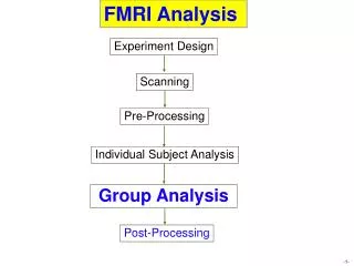
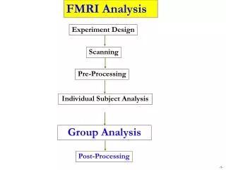
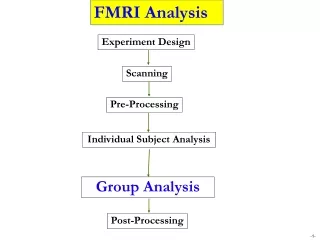
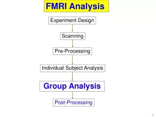
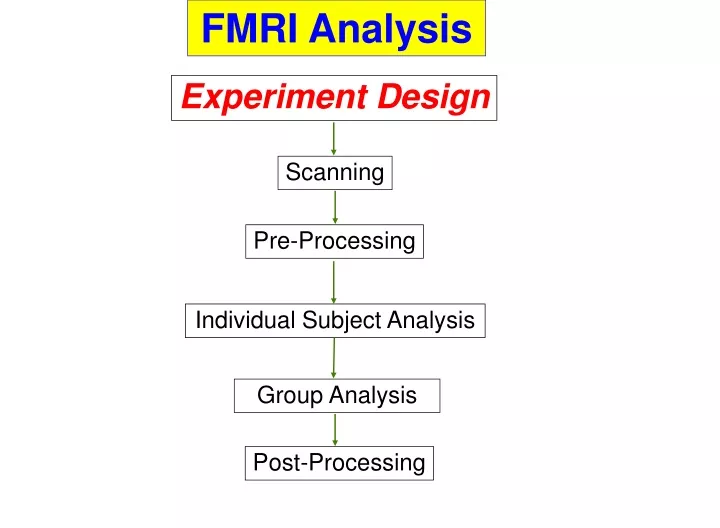
FMRI Analysis Experiment Design Scanning Pre-Processing Individual Subject Analysis Group Analysis Post-Processing
Scheme of the Talk • Design Types • Block • Event-related • Mixed • Players in Experiment Design • Intuitive Thinking • Usable bandwidth for FMRI data • Statistical Theory • Efficiency • Experiment Design in AFNI • AlphaSim and 3dDeconvolve • Summary • Miscellaneous
Design Types • Event-related design • Instant stimulus • Modeling options • Prefixed shape • Whatever fits: deconvolution • Various basis functions • Block design • Conditions with significant durations • Other terminologies: Epoch, box-car • Usually model with prefixed-shape HRF, but may also model with • deconvolution approach for flexible shapes • multiple events for each block: allow amplitude attenuation • Mixed design
Players in Experiment Design • Number of subjects (n) • Important for group analysis: inter-subject vs. intra-subject variation • Power roughly proportional to √n • Recommended: 20+; Current practice: 12 – 20 • Number of time points • Important for individual subject analysis • Power proportional to √DF • Limited by subject’s tolerance in scanner: 30-90 min per session • TR length • Shorter TR yields more time points (and potentially more power) • Power improvement limited by stronger temporal correlation and weaker MR signal • Shorter TR → shorter ISI → higher event freq → less power • Usually limited by hardware considerations
Players in Experiment Design • Design of the study • Complexity: factors, levels, covariate, contrasts of interest, balance of events/levels/subjects… • Design choices may limit statistical analysis options • Number of events per class • The more the better (20+), but no magic number • HRF modeling • Pre-fixed HRF, whatever fits, or other basis functions? • Event arrangement • How to design? How to define ‘best’ design? • Efficiency: achieve highest power within fixed scanning time • Inter-Stimulus Interval (ISI) and Stimulus Onset Asynchrony (SOA)
Intuitive Thinking • Classical HRF • Convolution in time = multiplication in frequency
Intuitive Thinking • Event frequency • Optimal frequency: 0.03 Hz (period 30 s) • Implication for block designs: optimal duration – about 15s • Upper bound: 0.20 Hz (5s) • Submerged in the sea of white noise • Implication for event-related designs: average ISI > 5s • Lower bound: 0.01 Hz (100 s) • Confounded with trend or removed by high-pass filtering • Implication for block designs: maximum duration about 50s* *Longer blocks could still be analyzed (see last slide) • Bandwidth: 0.01 – 0.15 Hz • Spread events within the frequency window (next topic)
Statistical Theory • Regression Model (GLS) • Y = Xb + e, X: design matrix with columns of regressors • General Linear testing • One test H0: c’b = 0 with c = (c0, c1, …, cp ) • t = c’b/√[c’(X’X)-1c MSE] (MSE: unknown but same across tests) • Signal-to-noise ratio • Effect vs. uncertainty • √(c’ (X’X)-1c): normalized standard deviation of contrast c’b • Efficiency = 1/√[c’(X’X)-1c]: Smaller → more powerful (and more efficient) • X’X measures the co-variation among the regressors: Less correlated regressors are more efficient and easier to tease regressors apart • X’X magnifies the uncertainty due to noise • Goal: find a design (X) that renders low norm. std. dev.
Statistical Theory • General Linear testing • Multiple tests: H01: c1’b = 0 with c1 = (c10, c11, …, c1p ),… H0k: ck’b = 0 with ck = (ck0, ck1, …, ckp ) • Efficiency (sensitivity): a relative value; dimensionless • in AFNI: 1/∑individual norm. std dev.’s • ∑individual efficiencies • Find efficient design • Minimizing ∑individual norm. std dev.’s • Minimax approach: Minimizing the maximum of individual norm. std dev.’s
Experiment Design in AFNI • AFNI programs for designing event-related experiments • RSFgen: Design X by generating randomized events • make_stim_times.py: convert stimulus coding to timing • 3dDeconvolve -nodata: calculate efficiency • Toy example: experiment parameters • TR = 2s, 300 TR’s, 3 stimulus types, 50 repetitions for each type • On average • One event of a type every 6 TR’s • ISI = 12 TR’s • frequency = 0.083 Hz
Experiment Design in AFNI • Toy example: Design an experiment and check its efficiency • TR = 2s, 300 TR’s, 3 event types (A, B, and C), 50 repetitions each • 3 tests of interest: A-B, A-C, and B-C • Modeling approach: prefixed or whatever fits? • Go to directory AFNI_data3/ht03 • 1st step: generate randomized events – script s1.RSFgen –by shuffling 50 1’s, 50 2’s, 50 3’s, and 150 0’s: RSFgen -nt 300 -num_stimts 3 \ -nreps 1 50 -nreps 2 50 -nreps 3 50 \ -seed 2483907 -prefix RSFstim. • Output: RSFstim.1.1D RSFstim.2.1D RSFstim.3.1D • Check the design by plotting the events • 1dplot `ls RSFstim.*.1D` &
Experiment Design in AFNI • Toy example: Design an experiment and check its efficiency • TR = 2s, 300 TR’s, 3 stimulus types, 50 repetitions for each type • 2nd step: Convert stimulus coding into timing (s2.StimTimes) make_stim_times.py -prefix stim -nt 300 -tr 2 -nruns 1 \ -files RSFstim.1.1D RSFstim.2.1D RSFstim.3.1D • Output: stim.01.1D stim.02.1D stim.03.1D • Check the timing files, e.g. • more stim.01.1D
Experiment Design in AFNI • Toy example: Design an experiment and check its efficiency • 3rd step: Calculate efficiency for each contrast (s3.Efficiency) set model = GAM # toggle btw GAM and 'TENT(0,12,7)‘ 3dDeconvolve -nodata 300 2 -nfirst 4 -nlast 299 \ -polort 2 -num_stimts 3 \-stim_times 1 "stim.01.1D" "$model" \ -stim_label 1 "stimA" \ -stim_times 2 "stim.02.1D" "$model" \ -stim_label 2 "stimB" \-stim_times 3 "stim.03.1D" "$model" \ -stim_label 3 "stimC" \ -gltsym "SYM: stimA -stimB" \ -gltsym "SYM: stimA -stimC" \ -gltsym "SYM: stimB -stimC" 3 regressors 3 contrasts
Experiment Design in AFNI • Toy example: Design an experiment and check its efficiency • Third step: Calculate efficiency for each contrast (s3.Efficiency) • Output: on terminal Stimulus: stimA h[ 0] norm. std. dev. = 0.1415 Stimulus: stimB h[ 0] norm. std. dev. = 0.1301 Stimulus: stimC h[ 0] norm. std. dev. = 0.1368 General Linear Test: GLT #1 LC[0] norm. std. dev. = 0.1677 General Linear Test: GLT #2 LC[0] norm. std. dev. = 0.1765 General Linear Test: GLT #3 LC[0] norm. std. dev. = 0.1680 • Efficiency is a relative number! Norm. Std. Dev. for 3 regressors Norm. Std. Dev. for 3 contrasts
Experiment Design in AFNI • Toy example: Design an experiment and check its efficiency • With TENT functions (modifying s3.Efficiency): TENT(0,12,7) (less efficient) Stimulus: stimA h[ 0] norm. std. dev. = 0.1676 ... h[ 6] norm. std. dev. = 0.1704Stimulus: stimB h[ 0] norm. std. dev. = 0.1694 ... h[ 6] norm. std. dev. = 0.1692Stimulus: stimC h[ 0] norm. std. dev. = 0.1666 ... h[ 6] norm. std. dev. = 0.1674General Linear Test: GLT #1 LC[0] norm. std. dev. = 0.5862 (0.1677)General Linear Test: GLT #2 LC[0] norm. std. dev. = 0.5826 (0.1765)General Linear Test: GLT #3 LC[0] norm. std. dev. = 0.5952 (0.1680) Norm. Std. Dev. for 21 regressors Norm. Std. Dev. for 3 contrasts: UAC or individual basis function (stim[[0..6]])?
Experiment Design in AFNI • Design search: Find an efficient design • TR = 2s, 300 TR’s, 3 stimulus types, 50 repetitions for each type • Script @DesginSearch: Parameters # TOGGLE btw the following 2 model parametersset model = GAM # toggle btw GAM and TENTset eff = SUM # toggle btw SUM and MAX # experiment parametersset ts = 300 # length of timeseriesset stim = 3 # number of input stimuliset num_on = 50 # time points per stimulus # execution parametersset iterations = 100 # number of iterationsset seed = 248390 # initial random seedset outdir = Results # move output to this directoryset TR = 2 # TR Length in secondsset ignore = 4 # number of TRs ignored set show = 10 # number of designs shown # Directories to store output filesset outdir = ${outdir}_${model}_$effset LCfile = $outdir/LCif ("$model" == "TENT") set model = ${model}'(0,12,7)'
Experiment Design in AFNI • Design search: Find an efficient design • Script @DesginSearch (continue): generate randomized designs # make sure $outdir exists...# compare many randomized designsforeach iter (`count -digits 3 1 $iterations`) # make some other random seed @ seed = $seed + 1 # create random order stim files RSFgen -nt ${ts} \ -num_stimts ${stim} \ -nreps 1 ${num_on} \ -nreps 2 ${num_on} \ -nreps 3 ${num_on} \ -seed ${seed} \ -prefix RSFstim${iter}. >& /dev/null
Experiment Design in AFNI • Design search: Find an efficient design • Script @DesginSearch (continue): Convert stimulus coding into timing make_stim_times.py -files RSFstim${iter}.1.1D \ RSFstim${iter}.2.1D RSFstim${iter}.3.1D \ -prefix stim${iter} \-nt 300 \-tr ${TR} \-nruns 1
Experiment Design in AFNI • Design search: Find an efficient design • Script @DesginSearch (continue): run regression analysis 3dDeconvolve \ -nodata ${ts} $TR \ -nfirst $ignore \ -nlast 299 \ -polort 2 \ -num_stimts ${stim} \ -stim_times 1 "stim${iter}.01.1D" "$model" \ -stim_label 1 "stimA" \ -stim_times 2 "stim${iter}.02.1D" "$model" \ -stim_label 2 "stimB" \ -stim_times 3 "stim${iter}.03.1D" "$model" \ -stim_label 3 "stimC" \ -gltsym "SYM: stimA -stimB" \ -gltsym "SYM: stimA -stimC" \ -gltsym "SYM: stimB -stimC" \ >& Eff${iter}
Experiment Design in AFNI • Design search: Find an efficient design • Script @DesginSearch (continue): Calculate norm. std. dev. for the design set nums = ( `awk -F= '/LC/ {print $2}' Eff${iter}` )if ("$eff" == "SUM") then# save the sum of the 3 normalized std devset num_sum = `ccalc -eval "$nums[1] + $nums[2] + $nums[3]"`echo -n "$num_sum = $nums[1] + $nums[2] + $nums[3] : " >> $LCfileecho "iteration $iter, seed $seed" >> $LCfileendif if ("$eff" == "MAX") then# get the max of the 3 normalized std devset imax=`ccalc -form int -eval \ "argmax($nums[1],$nums[2],$nums[3])"`set max = $nums[$imax]echo -n "$max = max($nums[1], $nums[2], $nums[3]) " >> $LCfileecho "iteration $iter, seed $seed" >> $LCfileendif
Experiment Design in AFNI • Design search: Find an efficient design` • Run the script tcsh @DesginSearch: Output The most 10 efficient designs are (in descending order):0.472800 = 0.1553 + 0.1596 + 0.1579 : iteration 092, seed 24839990.475300 = 0.1555 + 0.1610 + 0.1588 : iteration 043, seed 24839500.480300 = 0.1564 + 0.1632 + 0.1607 : iteration 020, seed 24839270.485600 = 0.1666 + 0.1560 + 0.1630 : iteration 006, seed 24839130.486800 = 0.1572 + 0.1615 + 0.1681 : iteration 044, seed 24839510.487200 = 0.1547 + 0.1663 + 0.1662 : iteration 100, seed 24840070.487400 = 0.1638 + 0.1626 + 0.1610 : iteration 059, seed 24839660.487700 = 0.1590 + 0.1605 + 0.1682 : iteration 013, seed 24839200.488700 = 0.1598 + 0.1659 + 0.1630 : iteration 060, seed 24839670.490500 = 0.1665 + 0.1635 + 0.1605 : iteration 095, seed 2484002 • Efficient design (under Results_GAM_SUM): 1dplot `ls Results_GAM_SUM/RSFstim092.*.1D` & Stimulus timing files are Results_GAM_SUM/stim092.*.1D
Experiment Design in AFNI • Design search: Find an efficient design • Script @DesginSearch (continue): try other options • TENT functions and summing set model = TENT set eff = SUM • GAM and minimax set model = GAMset eff = MAX • TENT functions and minimax set model = TENTset eff = MAX
Summary • Useful bandwidth: 0.01 – 0.15 Hz • Randomization • 2 kinds: sequence and ISI • Sequence randomization always good? • Experiment constraint • May not change efficiency much, but still good from other perspectives: Efficiency is not everything! • Neurological consideration that may not be considered through efficiency calculation • E.g., saturation, habituation, expectation, predictability, etc. • Nothing is best in absolute sense • Modeling approach: Pre-fixed HRF, basis function modeling, or else? • Specific statistical tests • Efficient design for one test is not necessary ideal for another
Miscellaneous • Dealing with low frequencies • Model drifting with polynomials (additive effect): 3dDeconvolve –polort • Order per 150s (~0.0067Hz) • High-pass filtering (additive effect): 3dFourier –highpass • Global mean scaling (multiplicative or amplifying effect) • Control condition • Baseline rarely meaningful especially for higher cognitive regions • If interest is on contrasts, null events are not absolutely necessary • If no control exists • High-pass filtering (additive effect): 3dFourier –highpass • Scaling by and regressing out white matter or ventricular signal • Multiple runs: concatenate or not • Analyze each run separately • Concatenate but analyze with separate regressors of an event across runs • Concatenate but analyze with same regressor of an event across runs