Download

1 / 57
570 likes | 707 Views
The Transmission-Switching Duality of Communication Networks. Tony T. Lee Shanghai Jiao Tong University The Chinese University of Hong Kong Xidian University, June 21, 2011. A Mathematical Theory of Communication BSTJ , 1948. C. E. Shannon. Contents. Introduction

E N D
The Transmission-Switching Duality of Communication Networks Tony T. Lee Shanghai Jiao Tong University The Chinese University of Hong Kong Xidian University, June 21, 2011
A Mathematical Theory of CommunicationBSTJ, 1948 C. E. Shannon
Contents • Introduction • Routing and Channel Coding • Scheduling and Source Coding
Reliable Communication • Circuit switching network • Reliable communication requires noise-tolerant transmission • Packet switching network • Reliable communication requires both noise-tolerant transmission and contention-tolerant switching
Quantization of Communication Systems • Transmission—from analog channel to digital channel • Sampling Theorem of Bandlimited Signal (Whittakev 1915; Nyquist, 1928; Kotelnikou, 1933; Shannon, 1948) • Switching—from circuit switching to packet switching • Doubly Stochastic Traffic Matrix Decomposition (Hall 1935; Birkhoff-von Neumann, 1946)
Transmission channel with noise Source information is a function of time, errors corrected by providing more signal space Noise is tamed by error correcting code Packet switching with contention Source information f(i) is a function of space, errors corrected by providing more time Contention is tamed by delay, buffering or deflection Noise vs. Contention Connection request f(i)= j 0111 0001 Message=0101 0101 0100 1101 Delay due to buffering or deflection
Transmission vs. Switching Shannon’s general communication system Received signal Message Signal Source Transmitter Channel capacity C Receiver Destination Temporal information source: function f(t) of time t Noise source Clos network C(m,n,k) Source Destination Input module Central module Output module nxm kxk mxn o o 0 0 0 n-1 n-1 Spatial information source: function f(i) of space i=0,1,…,N-1 N-n k-1 m-1 k-1 N-n N-1 N-1 Channel capacity = m Internal contention
Communication Channel Clos Network Noise Channel Coding Source Coding Contention Routing • Scheduling
Apple vs. Orange • 350mg Vitamin C • 1.5g/100g Sugar • 500mg Vitamin C • 2.5g/100g Sugar
Contents • Introduction • Routing and Channel Coding • Scheduling and Source Coding • Rate Allocation • Boltzmann Principle of Networking
Output Contention and Carried Load • Nonblocking switch with uniformly distributed destination address 0 0 • ρ: offered load • ρ’: carried load 1 1 N-1 N-1 • The difference between offered load and carried load reflects the degree of contention
Proposition on Signal Power of Switch • (V. Benes 63) The energyof connecting network is the number of calls in progress ( carried load ) • The signal power Sp of an N×N crossbar switch is the number of packets carried by outputs, and noise power Np=N- Sp • Pseudo Signal-to-Noise Ratio (PSNR)
Boltzmann Statistics 0 0 n0 = 5 1 3 4 6 7 a 1 1 b 2 2 0 5 n1 = 2 a d 3 3 c Micro State 2 n2 = 1 b,c 4 4 5 5 d Output Ports: Particles 6 6 Packet: Energy Quantum 7 7 energy level of outputs = number of packets destined for an output. ni = number of outputs with energy level packets are distinguishable, the total number of states is, = + + + N n n n Number of Outputs L 0 1 r
Boltzmann Statistics (cont’d) • From Boltzmann Entropy Equation • Maximizing the Entropy by Lagrange Multipliers • Using Stirling’s Approximation for Factorials • Taking the derivatives with respect to ni, yields • S: Entropy • W: Number of States • C: Boltzman Constant
Boltzmann Statistics (cont’d) • If offered load on each input is ρ, under uniform loading condition • Probability that there are i packets destined for the output • Carried load of output Poisson distribution
0 0 n-1 n-1 Clos Network C(m,n,k) k x k n x m m x n 0 0 0 0 0 0 • D = nQ + R • D is the destination address • Q =⌊D/n⌋ --- output module in the output stage • R = [D] n --- output link in the output module • G is the central module • Routing Tag (G,Q,R) 0 0 0 G G I Q n-1 n-1 m-1 k-1 k-1 m-1 D 0 0 nI 0 0 I G S I Q G nQ k-1 0 0 k-1 n(I+1)-1 n-1 m-1 Q G R nQ+R m-1 n-1 (n+1)Q-1 n(k-1) 0 n(k-1) 0 0 0 0 0 m-1 k-1 k-1 I G G Q nk-1 nk-1 n-1 m-1 m-1 n-1 k-1 k-1 Input stage Middle stage Output stage Slepian-Duguid condition m≥n
Clos Network as a Noisy Channel • Source state is a perfect matching • Central modules are randomly assigned to input packets • Offered load on each input link of central module • Carried load on each output link of central module • Pseudo signal-to-noise ratio (PSNR)
Noisy Channel Capacity Theorem • Capacity of the additive white Gaussian noise channel The maximum date rate C that can be sent through a channel subject to Gaussian noise is • C: Channel capacity in bits per second • W: Bandwidth of the channel in hertz • S/N: Signal-to-noise ratio
Planck's law can be written in terms of the spectral energy density per unit volume of thermodynamic equilibrium cavity radiation.
nxn kxk nxn kxk 0 0 0 0 k-1 n-1 k-1 n-1 C(n, n, k) C(k, k, n) Encoding output port addresses in C(k, k, n) Destination: D = kQ2 + R2 Output module number: Output port number: Encoding output port addresses in C(n, n, k) Destination: D = nQ1 + R1 Output module number: Output port number: Clos Network with Deflection Routing • Route the packets in C(n,n,k) and C(k,k,n) alternately Routing Tag = (Q1,R1, Q2,R2)
Loss Probability versus Network Length • The loss probability of deflection Clos network is an exponential function of network length
Shannon’s Noisy Channel Coding Theorem • Given a noisy channel with information capacity C and information transmitted at rate R • If R<C, there exists a coding technique which allows the probability of error at the receiver to be made arbitrarily small. • If R>C, the probability of error at the receiver increases without bound.
0 0 q q 1 1 p Binary Symmetric Channel • The Binary Symmetric Channel(BSC) with cross probability q=1-p‹½ has capacity • There exist encoding E and decoding D functions • If the rate R=k/n=C-δ for some δ>0. The error probability is bounded by • If R=k/n=C+ δ for some δ>0, the error probability is unbounded p
Edge Coloring of Bipartite Graph • A Regular bipartite graph G with vertex-degree m satisfies Hall’s condition • Let A ⊆ VI be a set of inputs, NA = {b | (a,b) ∈ E, a∈A} , since edges terminate on vertices in A must be terminated on NA at the other end.Then m|NA| ≥ m|A|, so |NA| ≥ |A|
Route Assignment in Clos Network 0 0 0 0 1 0 1 2 2 1 1 3 3 1 4 4 2 2 5 5 6 6 2 3 3 7 7 Computation of routing tag (G,Q,R)
RearrangeabeClos Network and Channel Coding Theorem • (Slepian-Duguid) Every Clos network with m≥n is rearrangeably nonblocking • The bipartite graph with degree n can be edge colored by m colors if m≥n • There is a route assignment for any permutation • Shannon’s noisy channel coding theorem • It is possible to transmit information without error up to a limit C.
LDPC Codes • Low Density Parity Checking (Gallager 60) • Bipartite Graph Representation (Tanner 81) • Approaching Shannon Limit (Richardson 99) VL: n variables VR: m constraints 0 x0 x1+x3+x4+x7=1 + Unsatisfied x1 1 x2 0 x0+x1+x2+x5=0 + x3 0 Satisfied 1 x4 x2+x5+x6+x7=0 + x5 1 Satisfied Closed Under (+)2 x6 0 x0+x3+x4+x6=1 + x7 1 Unsatisfied
Benes Network Bipartite graph of call requests 1 0 1 2 2 3 3 4 4 5 1 5 6 6 7 7 8 8 G(VL X VR, E) x1 + x1 + x2 =1 x2 x3 + x4 =1 + Input Module Constraints x3 x5 + x6 =1 + x4 x7 + x8 =1 + Not closed under + x5 x1 + x3 =1 + x6 x6 + x8 =1 Output Module Constraints + x7 x4 + x7 =1 + x8 x2 + x5 =1 +
Flip Algorithm • Assign x1=0, x2=1, x3=0, x4=1…to satisfy all input module constraints initially • Unsatisfied vertices divide each cycle into segments. Label them α and β alternately and flip values of all variables in α segments x1 0 x2 x1+x3=0 + + x1+x2=1 1 x3 0 x3+x4=1 x6+x8=0 + + x4 1 x5 0 x5+x6=1 x4+x7=1 + + x6 1 x7 x7+x8=1 x2+x5=1 0 + + x8 1 Input module constraints Output module constraints variables
Bipartite Matching and Route Assignments 1 1 2 2 Call requests 3 3 4 4 5 5 6 6 7 7 8 8 1 1 2 2 3 3 4 4 Bipartite Matching and Edge Coloring
Contents • Introduction • Routing and Channel Coding • Scheduling and Source Coding
Concept of Path Switching • Traffic signal at cross-road • Use predetermined conflict-free states in cyclic manner • The duration of each state in a cycle is determined by traffic loading • Distributed control N Traffic loading: NS: 2ρ EW: ρ W E NS traffic EW traffic S Cycle
0 0 1 1 2 2 Connection Matrix 0 0 0 0 0 1 Call requests 1 2 2 3 3 1 1 1 4 4 5 5 6 6 2 2 2 7 7 8 8 0 1 2 0 1 2
Path Switching of Clos Network 0 0 0 0 0 1 1 2 2 3 3 1 1 1 4 4 5 5 6 6 2 2 2 7 7 8 8 0 1 2 0 1 2 0 0 1 1 2 2 Time slot 2 Time slot 1
Capacity of Virtual Path • Capacity equals average number of edges Time slot 0 Virtual path 0 0 1 1 2 2 G1 Time slot 1 G1 U G2 0 0 1 1 2 2 G2
nxm kxk mxn 0 0 0 k-1 m-1 k-1 Contention-free Clos Network Input module (input queued switch) Central module (nonblocking switch) Output module (output queued Switch) o o n-1 n-1 o o n-1 n-1 Input buffer Predetermined connection pattern in every time slot Output buffer λij Source Buffer and scheduler Input module i Input module j Buffer and scheduler Destination Virtual path Scheduling to combat channel noise Buffering to combat source noise
Complexity Reduction of Permutation Space Subspace spanned by K base states {Pi} • Reduce the complexity of permutation space from N! to K Convex hull of doubly stochastic matrix K ≤ min{F, N2-2N+2}, the base dimension of C
Source Coding and Scheduling • Source coding: A mapping from code book to source symbols to reduce redundancy • Scheduling: A mapping from predetermined connection patterns to incoming packets to reduce delay jitter
Smoothness of Scheduling • Scheduling of a set of permutation matrices generated by decomposition • The sequence , ,……, of inter-state distance of state Pi within a period of F satisfies • Smoothness of state Pi with frame size F Pi Pi Pi Pi Pi F
Entropy of Decomposition and Smoothness of Scheduling • Any scheduling of capacity decomposition • Entropy inequality (Kraft’s Inequality) The equality holds when
P1 P2 P1 P3 P1 P2 P1 P4 Smoothness of Scheduling • A Special Case • If K=F, Фi=1/F, and ni=1 for all i, then for all i=1,…,F • Another Example Smoothness The Input Set The Expected Optimal Result
Optimal Smoothness of Scheduling • Smoothness of random scheduling • Kullback-Leibler distance reaches maximum when • Always possible to device a scheduling within 1/2 of entropy
Source Coding Theorem • Necessary and Sufficient condition to prefix encode values x1,x2,…,xN of X with respective length n1,n2,…nN • Any prefix code that assigns ni bits to xi • Always possible to device a prefix code within 1 of entropy (Kraft’s Inequality)
Huffman Round Robin (HuRR) Algorithm Initially set the root be temporary node Px, and S = Px…Px be temporary sequence. Step1 Apply the WFQ to the two successors of Px to produce a sequecne T, and substitute T for the subsequence Px…Px of S. Step2 If there is no intermediate node in the sequence S, then terminate the algorithm. Otherwise select an intermediate node Px appearing in S and go to step 2. Step3 1 PZ 0.5 PX PY 0.25 0.25 P1 P2 P3 P4 P5 0.5 0.125 0.125 0.125 0.125 Huffman Code logarithm of interstate time = length of Huffman code
Performance of Scheduling Algorithms Better Performance