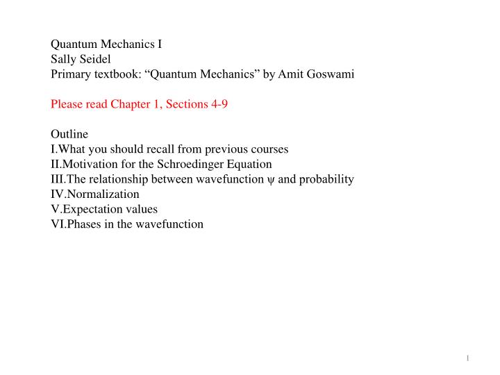
Quantum Mechanics I Sally Seidel Primary textbook: “Quantum Mechanics” by Amit Goswami

1. Quantum Mechanics I • Sally Seidel • Primary textbook: “Quantum Mechanics” by Amit Goswami • Please read Chapter 1, Sections 4-9 • Outline • What you should recall from previous courses • Motivation for the Schroedinger Equation • The relationship between wavefunction ψ and probability • Normalization • Expectation values • Phases in the wavefunction

2. 10 facts to recall from previous courses • Fundamental particles (for example electrons, quarks, and photons) have all the usual classical properties (for example mass and charge) + a new one: probability of location. • Because their location is never definite, we assign fundamental particles a wavelength. • Peak of wave – most probable location • length of wave – amount of indefiniteness of location • Wavelength λ is related to the object’s momentum p • The object itself is not “wavy”...it does not oscillate as it travels. What is wavy is its probability of location. Planck’s constant 4.13 x 10-15 eV-sec

3. Example of an object with wavy location probability distribution Consider a set of 5 large toy train cars joined end to end. Each car has a lid and a door leading to the next car. Put a mouse into one box and close the lid. The mouse is free to wander among boxes. At any time one could lift a lid and have a 20% chance to find the mouse in that particular car. Now equip Boxes 2 and 4 with mouse repellent Equip Boxes 1, 3, and 5 with cheese

4. A diagram on the outside of the boxes shows how likely it is that the mouse is in any of the boxes. Now the probability of finding the mouse is not uniform in space: maxima are near the cheese, minima are near the poison. Probability very likely sometimes not likely sometimes very likely Position • Conclude: • the mouse does not look like a wave---it looks like a mouse • the mouse does not oscillate like a wave---it moves like a mouse • but the map of probable locations for the mouse is shaped like a wave

5. The situation for the electron or photon is almost the same, except • for the mouse example, Probability = Amplitude • for the electron (or any quantum mechanical object, • Probability = (Amplitude)*(Amplitude) • As with all waves, wavelength λ is related to frequency υ: • λυ= velocity of wave • 6. QM says that the λ ( or υ) is also related to the energy: • E=hυ • Special relativity says that total E and momentum p are also related by c = 3 x 108 m/s rest mass of the object

6. QM says that every object in the universe is associated with a mathematical expression that encodes in it every property that it is possible to know about the object. • This math expression is called the object’s wavefunction ψ. • As the object moves through space and time, some of its properties (for example location and energy) change to respond to its external environment. • So ψ has to track these • Conclude: ψ has to include information about the environment of the particle (for example location x, time t, sources of potential V) • 10. So if you know the ψ of the object, you can find out everything possible about it. • The goal of all QM problems is: given an object (mass m, charge Q, etc.) in a particular environment (potential V), find its ψ. The way to do this (in 1-dimension) is to solve the equation its charge, mass, location, energy... The Schroedinger Equation

7. II. Motivation for the Schroedinger Equation We can develop the Schroedinger Equation by combining 6 facts: FACT 1: The λ and p of the ψ produced by this equation must satisfy λ=h/p. FACT 2: The E and υ of the ψ must satisfy E=hυ. FACT 3: Total energy = kinetic energy + potential energy Etota l= KE + PE Restricting ourselves to non-relativistic problems, we can rewrite this as Etotal = p2/2m + V. (For relativistic problems, we would need ). FACT 4: Because a particle’s energy, velocity, etc, depend on any force F it experiences, the equation must involve F. Insert this as a V-dependence through To simplify initially, consider only cases where V = constant = V0. Later we will generalize to V=V(x,y,z,t).

8. FACT 5: The only kind of wave that is present in the region of a constant potential is an infinite wave train of constant λ everywhere. • Example: • An ocean wave over the flat ocean floor extends in all directions with constant amplitude and λ. • When the wave reaches a change in floor level (i.e. a beach) then its structure changes. • Conclude: if V = constant, • Recall that the definition of a wave is an oscillation that maintains its shape as it propagates. For constant velocity v, “x-vt” ensures that as t increases, x must increase to maintain the arg=(x-vt)= constant. This is a rightward-traveling wave. k has units 1/length to make the argument of the cos dimensionless cos or sin indicate the wave shape.

9. Again Rewrite this as Then FACT 6: ψ represents a particle and wave simultaneously. Waves interfere. This means if we combine the amplitudes of 2 waves (A(ψ1) and A(ψ2)), we get A(ψTotal) = A(ψ1) + A(ψ2). That is...add the first powers of the ψ1 and ψ2 amplitudes, not functions that are more complicated. Conclude: if we want the Schroedinger Equation to produce a wavelike ψ, then it too must include only first powers of ψ...that is, ψ, dψ/dx, dψ/dt, etc., but NOT, for example, ψ2. units are So call kv = ω.

10. Now use all 6 facts to construct the Schroedinger Equation: Notice we are already using FACT 4 (i.e. V is included. Consider the simplified case V = constant = V0. This implies Recall this produces an infinite, single-λ wave.

14. III. The connection between ψ and probability Max Born proposed (1926) that the probability of finding a particle at a specific location x at time t, Prob(x,t) = ψ*ψ. Justification: If the particle that ψ describes is assumed to last forever [this must later be revised by Quantum Field Theory] then the probability associated with finding it somewhere must always be 1. So probability must have an associated continuity equation like the one that applies to electric charge. In electricity and magnetism: electric current density electric charge density

15. We need an analogous expression to describe • probability density ρProb and • probability current JProb which can flow in space but remain conserved. • Assume ρProb and Jprob involve ψ somehow, but in an unspecified function. • Plan: • Use the only equation we have for ψ: the Schroedinger Equation • Manipulate it to get the form

17. IV. Normalizing a wavefunction Recall that when we were deriving the Schroedinger Eq. for a free particle, we got to this step: We guessed ψ=δcos(kx-ωt)+γsin(kx-ωt) We found that γ=±iδ So ψ = δcos(kx-ωt) ± iδsin(kx-ωt) =δ[cos(kx-ωt) ± isin(kx-ωt)] Although this function corresponds to ψfree, all ψ’s have a “δ”. Next goal: find a general technique for obtaining δ. This is called normalizing the wavefunction. 2 options correspond to waves traveling right and left. We can choose either one. As-yet unspecified overall amplitude

18. To find δ, recall P(x,t) = ψ*ψ The sum of probabilities of all possible locations of the particle must be 1.

19. V. Expectation values Although particle is never in a definite location, it is more likely to be in one location than others, if any potential V is active. Recall the definition of a weighted average position: This is the “expectation value of x” By convention, place x between ψ’s If ψ has been normalized, this denominator is 1.

21. Please read Goswami Chapter 2. • Outline • Normalizing a free particle wavefunction • Acceptable mathematical forms of ψ • The phase of the wavefunction • The effect of a potential on a wave • Wave packets • The Uncertainty Principle

24. II Acceptable mathematical forms of wavefunctions ψ must be normalizable, so must be a convergent integral- i.e., at minimum, require A ψ that satisfies this is called “square integrable.”

25. III The phase of the wavefunction FACT 1: We cannot observe ψ itself; we only observe ψ*ψ. So overall phase is physically irrelevant. FACT 2: The relative phase of two ψ’s in the same region affects the probability distribution, which is measurement, through superposition: Suppose ψ1 = Aeiα and ψ2 = Beiβ, where A and B are real. ψtot = Aeiα + Beiβ = eiα[A+Bei(β-α)], so Prob=ψ*ψ=[A+Bei(β-α)][A+Be-i(β-α)]=A2+B2+AB[ei(β-α)+e-i(β-α)]= A2 + B2 + 2ABcos(β-α) FACT 3: The flow of probability depends on both the amplitude and the phase: Consider ψ=Aeiα where A can be complex.

26. phase dependence amplitude dependence

27. IV The effect of a potential upon a wave If everywhere in the universe, V were constant, all particle/waves would be free and described by ψfree=e i(kx-ωt), an infinite train of constant wavelength λ. If somewhere V≠constant, then in that region ψ will be modulated. schematic potential schematic wavefunction response A modulated wave is composed of multiple frequencies (i.e., Fourier components) that create beats or packets.

28. V. Wave packets The more Fourier component frequencies there are constituting a wave packet, the more clearly separated the packet is from others. Specific requirements on a packet: To achieve a semi-infinite gap on each side of the packet (i.e. a truly isolated packet/particle), we need an infinite number of waves of different frequencies. Each component is a plane wave To center the packet at x = x0, modify so at x≅x0, all the k’s (ν’s) superpose constructively. 4. To tune the shape of the packet, adjust the amplitude of each component separately---so

29. A(k) is called the Fourier Transform of ψ(x) infinite number of ν’s (k’s)

30. VI. The Uncertainty Principle The shape of a packet depends upon the spectrum of amplitudes A(k) of its constituent Fourier components. Examples of possible spectra: Note this is the A(k) not the ψ(x). A(k) k A(k) A(k)=δ(k-k0) Dirac delta k

31. Each A(k) spectrum produces a different wavepacket shape, for example • . • versus • Qualitatively it turns out that • large number of constituent k’s in the A spectrum (=large “Δk”) produces a short packet (small “Δx”). • So • So ΔpΔx cannot be arbitrarily small for any wave packet. • We begin to see that the Uncertainty Principle is a property of all waves, not just a Quantum Mechanical phenomenon.

32. The proportionality in is qualitative at this point. To derive the Uncertainty Principle from this, we need to know: a precise definition of Δp a precise definition of Δx what is the smallest combined choice of ΔpΔx (or ΔkΔx) that is geometrically possible for a wave. To answer these, use the Gaussian wave packet in k-space to answer the questions above, in the reverse order. A(k) k

33. Find this amplitude by normalization later.

34. Answer to (2)--- “What is Δx?” : For all A(k) spectra, the precise definition of Δx is For simplicity, choose center of the packet at x0 = 0. Then

37. Please read Goswami Chapter 3. • Outline • I. Phase velocity and group velocity • II. Wave packets spread in time • III. A longer look at Fourier transforms, momentum conservation, and packet dispersion. • Operators • Commutators • VI. Probing the meaning of the Schroedinger Equation

38. Phase velocity and group velocity • A classical particle has an unambigous velocity Δx/Δt or dx/dt because its “x” is always perfectly well known. • A wave packet has several kinds of velocity: • In general vphase ≠ vgroup. Which velocity is related to the velocity of the particle that this wave represents? vgroup, the rate of travel of the peak of the envelope. vphase, the rate of travel of the component ripples

39. Recall a traveling wave packet is described by • Bear in mind the definitions • k = 2π/λ “inverse wavelength” and • ω = 2πυ “angular frequency” • Recall ω = ω(k). • If the packet changes shape as it travels, the function may be complicated. • If the packet changes shape rapidly and drastically, the notion of a packet with well-defined velocity becomes vague. • For clarity, consider only those packets that do not change shape “much” as they travel. • For them, ω(k)=constant + small terms proportional to some function of k. • Taylor expand ω about some k=k0. • Plug this into ψ:

40. This is identical to ψ(x,0) except the position of the packet is shifted by so that must be the velocity of the packet: This is an overall phase which has no meaning in ψ*ψ, so forget it.

41. Conclude: vgroup = dω/dk is the velocity of the packet envelope AND of the associated particle. vphase = ω/k is usually different from dω/dk. Notice

42. II. Wave packets spread in time • The lecture plan: • Recall ψGeneral A’s(x,t =0) • Specialize to ψGaussian A’s(x,t =0) • Extrapolate from x to x-vt, so eikxei(kx-ωt) • Find P(x,t)=ψ*(x,t)ψ(x,t). • We will find that |ψ(x,t)|2 is proportional to exp(-x2/(stuff)2). • Since the width of ψ is defined as the distance in x over which ψ decreases by e, this “stuff” is the width. • We will see that the “stuff” is a function of time. • Carry out the plan...

44. call this T, the characteristic spreading time. Notice this is Δx(t=0).

45. Conclusions: • The width Δx of the probability distribution increases with t, i.e., the packet spreads. • This only works because the amplitudes A are time-independent, i.e., the A(k) found for ψ(t=0) can be used for ψ(all t). The A(k) distribution is a permanent characteristic of the wave. • Notice the “new x”: • The group velocity naturally appears because this Δx describes a property of the packet as a whole. • (4) Recall the A(k) are not functions of t, so • Prob(k,t) = A*A does not have time-dependence, so Δp does not spread as Δx does. • This is momentum conservation.

46. A longer look at Fourier transforms, momentum conservation, and packet dispersion

48. These ω’s are the frequencies of the Fourier components. The components are plane waves---the ψ’s of free particles.

49. Operators • Recall earlier we wanted • but we needed to represent p as a function of x. How to find this representation: • Recall the wavefunction for a free particle is ψ = ei(kx-ωt). • Notice • This says: if ψ represents a free particle, any time we have “pψ”, we can replace it with

50. Q. What if ψ is NOT a free particle?...what if ψ is influenced by a potential V so is a packet? Ans. The packet is a superposition of free particle states, so the replacement is still valid. Use a similar method to find the operator for energy E: Begin with is ψfree = ei(kx-ωt). Notice