Download
1 / 28
280 likes | 412 Views
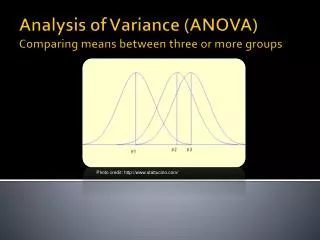
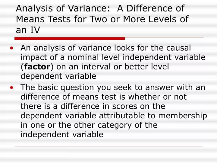
Analysis of Variance: A Difference of Means Tests for Two or More Levels of an IV. An analysis of variance looks for the causal impact of a nominal level independent variable ( factor ) on an interval or better level dependent variable

E N D
Analysis of Variance: A Difference of Means Tests for Two or More Levels of an IV • An analysis of variance looks for the causal impact of a nominal level independent variable (factor) on an interval or better level dependent variable • The basic question you seek to answer with an difference of means test is whether or not there is a difference in scores on the dependent variable attributable to membership in one or the other category of the independent variable
Types of Difference of Means Tests • Varieties of test for difference of means where there is a single independent variable or factor • t-test: two levels of the independent variable • What is the impact of gender (M, F) on annual salary? • Analysis of Variance (ANOVA): Two or more levels or conditions of the independent variable • What is the impact of ethnicity (Hispanic, African-American, Asian-Pacific Islander, Caucasian, etc) on annual salary? • ANOVA models can be fixed or random • Fixed model overwhelmingly used • Effects obtained in the fixed model only generalizable to other identical levels of the factor studied (e.g., only to treatments A, B, C such as online vs. classroom instruction) • Effects obtained in the random model generalizable to a wider range of values of the IV than just the three levels • Time of day could be a random factor and you randomly decide to compare classes taught at 8 am, noon, and 3 pm but these values are “replaceable” by other randomly drawn values or you could add more time periods • Subject matter or teacher could be another random factor
Repeated Measures and Analysis of Covariance • In a repeated measuresANOVA design, the same Ss are tested across different levels of the factor (example, time 1, time 2, time 3, …time n) • In an analysis of covariance, we statistically control for the effects of pre-existing differences among subjects on the DV of interest (e.g. controlling for the effects of an individual’s computer experience in evaluating impact of presence or absence of narrative on enjoyment of computer game play)
More on Tests of Difference of Means: Analysis of Variance with Two Independent Variables (Factors) Two-way ANOVA: two or more levels of two IVs or factors • What is the impact of diet type and educational attainment on pounds lost in six months, and how do they interact? • This data suggests two significant factors that behave the same way regardless of the level of the other factor (Diet C is always better, post grad always better); don’t interact Average pounds lost as a function of educational attainment and diet type
When Factors Interact In this data set there seems to be an interaction between diet type and educational attainment, such that Diet C is more effective for people with lower educational attainment, Diet A works better for people with high attainment, and Diet B works equally well regardless of educational attainment. Impact of one factor depends on the level of the second factor Average pounds lost as a function of educational attainment and diet type
Single-factor ANOVA Example (one Independent Variable) • Suppose you believed that interviewer status (a manipulated variable in which you systematically varied the dress of the same interviewer across the conditions, high medium, and low would have an effect on interviewee self-disclosure, such that the amount of disclosure of negative personal information would vary across conditions. (The null hypothesis would be that the interviewees all came from the same population of interviewers) Let’s say you conducted your study and got the data on the right, where higher scores equal more self-disclosure Self-disclosure scores for 12 subjects; 4 subjects in each of three interviewer conditions
Some Typical Data for ANOVA The sum over all rows and columns, denoted as ∑∑Xij, = 36 i j (That’s 8 + 12 + 16) The grand mean, denoted Xij, is 3 (That’s 2 + 3 + 4 divided by 3) The overall N is 12 (That’s 4 subjects in each of three conditions)
Partitioning the Variance for ANOVA: Within and Between Estimates: how to obtain the test statistic, F, for the difference of means • To obtain the F statistic, we are going to make two estimates of the common population variance, σ2 • The first is called the “within” estimate, which will be a weighted average of the variances within each of the three samples. This is an unbiased estimate of σ2 and is an estimate of how much of the variance in self-disclosure scores is attributable to more or less random individual differences • The second estimate of the common variance σ2 is called the “between” (or “among”) estimate and it involves the variance of the sample means about the grand mean. This is an estimate of how much of the variation in self-disclosure scores is attributable to the levels of the factor (interviewer status). The “between” refers to between-levels variation • If our factor has a meaningful effect the “between estimate” should be large relative to the “within estimate”; that is, there should be more variation between the levels of interviewer status than within them
Meaning of the F Statistic, the Statistic used in ANOVA • The sampling distribution of the F ratio will be used to determine how probable it is that our obtained value of F was due to sampling error • The null hypothesis would be that the population means for the three treatment levels would not differ • If the null hypothesis is false, and the population means are not equal, then the F ratio will be greater than unity (one). Whether or not the means are significantly different will depend on how large this ratio is • There is a sampling distribution for F (see p. 479 in Kendrick) called the “Distribution of the Critical Values of F”; note that there are separate tables for the .05 and .01 confidence levels). (see also the next slide) • The columns refer to n1, the DF of the between groups estimate (K-1, where K is the number of conditions or treatments of the independent variable) and the rows refer to n2, the DF of the within groups estimate (N (total) – K) • For our example n1, the between DF, would be 2 and n2, the within DF, would be 9
Partitioning the Variation in ANOVA • The twelve self-disclosure scores we have obtained vary quite a bit from the grand mean of all the scores, which was 3 • The total variation is the sum of the squared deviations from the grand (overall) mean. This quantity is also called the “total sum of squares” or the total SS. Its DF is equal to N-1, where N is the total over all the cases. The total variation has two components • The within sum of squares: the sum of the squared deviations of the individual scores from their own category (group) mean. We divide this by the df (N-K) to obtain the within estimate. This represents the variability among individuals within the sample • The between (among) sum of squares: this is based on the squared deviations of the means of the IV levels from the grand mean, and is a measure of the variability between the conditions. We want this quantity to be big! We divide the betwenn SS by the df K-1 to get the between estimate • The within and between estimates are also called the between and within “mean squares”
A Hand Calculation of ANOVA: Obtaining the Between and Within Estimates • To get the between estimate, the first thing we calculate is the between sum of squares: • We find the difference between each group mean and the grand mean (3), square this deviation, multiply by the number of scores in the group, and sum these quantities
Between Estimate Calculations • So we have • High Status: 2-3 squared X 4 = 4 • Medium Status: 3-3 squared X 4 = 0 • Low Status: 4-3 squared X 4 = 4 • So the between sum of squares = 4+ 0 + 4 = 8 • And the between estimate is obtained by dividing the between SS by the between degrees of freedom, K-1 • Thus the between estimate is 8/2 or 4 ∑∑=36
Calculating the Total Sum of Squares • The next thing we calculate is the total sum of squares. This figure is obtained by summing the squared deviations of each of the individual scores from the grand mean of 3. So the total sum of squares is 3-3 squared plus 2-3 squared plus 1-3 squared plus 2-3 squared plus 3-3 squared plus 4-3 squared…. plus 4-3 squared = 14
Calculating the Within Estimate • Finally, we calculate the within sum of squares. We obtain that by subtracting the between SS (8) from the total SS (14). So the within SS = 6. And the within estimate is obtained by dividing the within SS by its DF, so the within estimate or within mean square is 6/(N-k) or 6/9 or .667 • Recall that for the null hypothesis, that the population means for the three conditions are equal, to be true, the between estimate should equal the within estimate, yet our between estimate is very large in relation to the within estimate. This is good; it means that the variance “explained” by the status manipulation is much greater than what individual differences alone can explain • See the table on the next page which shows the estimates for the different sources of variation
Basic Output of an ANOVA Called “mean squares” The between and within estimates are obtained by dividing the between and within SS by their respective DFs.The F statistic is obtained by dividing the between estimate by the within estimate (4/.667 = 6) The obtained value of F tells us that the variation between the conditions is much greater than the variation within each condition. We look up the F statistic in the table with 2 DF (conditions minus 1) in the numerator and 9 DF (total N minus number of conditions) in the denominator and we find that we need a F of 4.26 to reject the null hypothesis at p < .05. (see next slide)
Looking up the F Value in the Table of Critical Values of F With our obtained F of 6 we can reject the null hypothesis
ANOVA in SPSS • Now let’s try that in SPSS. Go here to download the data file disclosure.sav and open it in SPSS • In Data Editor go to Analyze/Compare Means/One-Way Anova • Move the Interviewer Status variable into the Factor window and move the Self-Disclosure variable into the Dependent List window • Under Options select Descriptive, then press Continue and then OK • Compare the results in your Output Window to the hand calculations and to the next slide
SPSS Output, One-Way ANOVA The results of this analysis suggest that interviewer status has a significant impact on interviewee self-disclosure, F (2,9) = 6, p < .05 ( or p = .022)
Planned Comparisons vs. Post-hoc Comparison of Means • Even if we have obtained a significant value of F and the overall difference of means is significant, the F statistic isn’t telling us anything about how the mean scores varied among the levels of the IV. Fortunately, we know that this will be the case in advance, and so we can plan some comparisons between the pairwise group means that we will specify in advance. These are called planned comparisons. • Alternatively, we can compare the means of the groups on a pair-wise basis after the fact • Doing comparison-of-means tests after the fact, when we have had time to check out the means and see what direction they’re tending (for example, we can look and see that there was more disclosure to the low-status interviewer than to the high-status interviewer), it’s not really the done thing to allow a low confidence level like .10 when we know the direction of the results. We should use a more conservative alpha region in order to reduce the risk of Type I error (rejecting a true null hypothesis)
Post-hoc Tests in SPSS • In SPSS data editor, make sure you have the disclosure.sav data file open • Go to Analyze/Compare Means/One-Way Anova • Move Interviewer Status into the Factor box (this is where the IVs go) • Move Self-disclosure into the Dependent List box • Under Options, select Descriptive, Homogenity of Variance test, and Means Plot, and click Continue • Under Post Hoc, click Sheffé and Tukey and set the confidence interval to .05, then click Continue and OK • Compare your output to the next slide
Output for Post-Hoc Comparisons Variances are equal Important! Both Tukey and Sheffé tests show significant differences between high and low status condition but not between medium status and other two conditions. Tukey can only be used with groups of equal size. Sheffé critical value (test statistic that must be exceeded) = k-1 times the critical value of F needed for the one-way anova at a particular alpha level. If variances are unequal by Levene, use the Tamhane’s T2 test for post-hoc comparisons
Writing up Your Result • To test the hypothesis that interviewer status would have a significant effect on interviewee self-disclosure, a one-way analysis of variance was performed. Levene’s test for the equality of variances indicated that the variances did not differ significantly across levels of the independent variable (Levene statistic = 000, df = 2, 9, p=1.00). Interviewer status had a significant main effect on interviewee self-disclosure (F (2,9) = 6, p = .022). Sheffe’ post-hoc tests indicated that there were significant differences between mean levels of disclosure for subjects in the high status (M = 2) and low status (M = 4) conditions (p =.022), suggesting an inverse relationship between interviewer status and interviewee disclosure. Subjects disclosed more to the low-status interviewer.
More SPSS ANOVA • Using the general social survey data, let’s test the hypothesis that one’s father’s highest earned degree has a significant impact on one’s current socio-economic status • Download the socialsurvey.sav file and open it in Data Editor • Go to Analyze/Compare Means/One-Way Anova • Move Father’s Highest Degree into the Factor box and move Respondent Socioeconomic Index into the Dependent List box • Under Options, select Descriptive and Homogeneity of Variance test and click Continue • Under Post Hoc select Sheffé and set the significance level to .05, select Continue and then OK • Compare your output to the next slides
Using the General Linear Model in SPSS • Now we are going to redo the same analysis but with a few more bells and whistles. This time, for example, we are going to get measures of the effect size (impact of the IV, father’s highest degree) on the DV, respondent’s SES, and we will also get a power estimate • In the Data Editor, make sure your socialsurvey.sav file is open • Go to Analyze/General Linear Model/Univariate (in the case of ANOVA, univariate means you only analyze one DV at a time) • Put Father’s Highest Degree into the Fixed Factor box and Respondent’s SES into the Dependent Variable box • Under Post Hoc, move padeg (shorthand for Father’s Highest Degree) into the Post Hoc Tests for box and under Equal Variances assumed select Sheffé (we can do this because we already know that the variances are not significantly different from our previous analysis) and click Continue • Click on Options and move padeg into the Display Means for box • Under Display, click on Descriptive Statistics, Estimates of Effect Size, and Observed Power, and set the significance level to .05. Click continue and then OK. Compare your result to the next slide
SPSS GLM Output, Univariate Analysis Note that we have all the power required to detect an effect = Independent variable Note partial eta squared which is the ratio of the between-groups SS to the sum of the between groups SS and the error SS. It describes the amount of variation in the dependent variable explained by the independent variable (Father’s highest degree). In this case the amount of variation accounted for, about 7%, is not very impressive despite a significant result corrected means that the variance accounted for by the intercept has been removed
SPSS GLM Output, Univariate Analysis, cont’d Note confidence intervals around the mean difference estimates. These intervals should not contain zero (recall that the null hypothesis is of no differences on the dependent variable between levels of the IV) Note also above that some of the confidence levels around the category means themselves contain the mean of the other category. So this sort of data should be studied as well as significance tests