Download

1 / 20
200 likes | 206 Views
Friday 11 February 2011. Lecture 12: Image Processing. Reading Ch 7.1 - 7.6. Last lecture: Earth-orbiting satellites. Image Processing Because of the way most remote-sensing texts are organized, what strikes most students is the vast array of algorithms with odd names

E N D
Friday 11 February 2011 Lecture 12: Image Processing Reading Ch 7.1 - 7.6 Last lecture: Earth-orbiting satellites
Image Processing Because of the way most remote-sensing texts are organized, what strikes most students is the vast array of algorithms with odd names and obscure functions What is elusive is the underlying simplicity. Many algorithms are substantially the same – they have similar purposes and similar results
Image Processing • There are basically five families of • algorithms that do things to images: • Radiometric algorithms • change the DNs • Calibration • Contrast enhancement • 2) Geometric algorithms • change the spatial arrangement of pixels or adjust DN’s based on their neighbors’ values • Registration • “Visualization” • Spatial-spectral transformation • Spatial filtering
Contrast stretching & calibration Enhancement: Imagine a DN histogram centered at 75 DN and running from 50 to 100. In lab, you would move sliders to 50 and 100 DN to display it well. Mathematically, you are saying that (100-50)=50 DN’s are going to be packed into 256 gray levels, DN’. Furthermore, the center of the distribution will be 128 DN’. DN’=gain *DN+offset So the amplification factor or gain will be 256/(100-50)=5.12: DN’=5.12*DN+offset Now if we take 75 DN, the central value that we want to be 128, and multiply it by 5.12, we get 384 DN’, so we need to subtract 256 to get the right answer: DN’=5.12*DN-256. Check: DN’=5.12*50-256 = 0; DN’=5.12*75-256=128; DN’=5.12*100-256=156 Calibration: We measure radiance in DNs, but we want to know reflectance. So we can take a known target (say, black and white cardboard with reflectances measured in the lab of 5 and 25%) and image them to find out what radiance DN’s they give (say, 13 and 47, respectively). Then we can do a controlled contrast stretch to give the image in reflectance units: Now, the gain will be DDN /Drefl = (25-5)/(47-13)=0.59 (That is, refl=0.59*DN+offs, and we find offset by Knowing 0.59*13=5, or offset = 5-0.59*13=5-7.67=-2.67, so refl=0.59*DN-2.67. Check: 25=0.59*47-2.67=25.06 (roundoff) Calibration is just a special kind of contrast stretch
Geometric registration Pixel locations in original and corrected images DN values in corrected image are found by interpolation from the nearest neighbors in the acquired image Acquired image, distorted Map with locations of control points
Image Processing 3) Spectral analysis algorithms are based on the relationship of DNs within a given pixel Color enhancement Spectral transformations (e.g., PCA) Spectral Mixture Analysis 4) Statistical algorithms characterize or compare groups of radiance data Estimate geophysical parameters Spectral similarity (classification, spectral matching) Input to GIS
Image Processing 5) Modeling calculate non-radiance parameters from the radiance and other data Estimate geophysical parameters Make thematic maps Input to GIS
Image Processing There is a dazzling array of things for the future professional to become familiar with We’re trying to over-simplify it to begin with Most algorithms are handled pretty well in most remote-sensing texts. Spectral Mixture Analysis is an exception, so… - we’ll look at Spectral Mixture Analysis next lecture
Image Processing Sequence(single image) Raw image data 1. Image display/inspection 2. Instrument calibration Image rectification, cartographic projection, registration, geocoding 3. Pre-processing 4. Atmospheric compensation Pixel illumination-viewing geometry (topographic compensation) 5. Working image data
Working image data Product Image Processing Sequence(single image) 6. Further image processing 7. Spectral analysis Selection of training data/endmembers 8. Processing Initial classification or other type of analysis 9. Interpretation/verification or further analysis 10.
Ratios in 2-space TM4 TM3 TM4 Ratio – 11 sunlit Ratio – 1.5 Ratio - 1.1 shadowed shadow TM3
Ratios The Vegetation Index (VI) = DN4/DN3 is a ratio. Ratios suppress topographic shading because the cos(i) term appears in both numerator and denominator.
NDVINormalized Difference Vegetation Index DN4-DN3 is a measure of how much chlorophyll absorption is present, but it is sensitive to cos(i) unless the difference is divided by the sum DN4+DN3.
Dimension rotation y y’ x’ 0.7x,0.7y -0.7x, 0.7y + x y 0.5x,0.87y -087x,0.5y + x y x’ 0x,1y + x y’ -1x,0y
Principal Component Analysis (PCA) • Designed to reduce redundancy in multispectral bands • Topography - shading • Spectral correlation from band to band • Either enhancement prior to visual interpretation or pre-processing for classification or other analysis • Compress all info originally in many bands into fewer bands • http://en.wikipedia.org/wiki/Principal_component_analysis
Principal Component Analysis (PCA) - The math behind the button [ ] PC1 PC2’ = In the simple case of 45º axis rotation, Finding q [ ] [ ] [ ] [ ] cos q sin q -sin q cos q DN1’ DN2’ DN1 DN2 n11 n12 n21 n22 = cov = q = 45º Cov’=RTcovR; cov’ is the matrix having eigenvalues as diagonal elements and RT is the transpose of R. Eigenvalues can be found by diagonalizing cov. R has eigenvectors as column vectors http://www.cs.otago.ac.nz/cosc453/student_tutorials/principal_components.pdf http://en.wikipedia.org/wiki/Principal_component_analysis
Principal Component Analysis In the simple case of 45º axis rotation, The rotation in PCA depends on the data. In the top case, all the image data have similar DN2/DN1 ratios but different intensities, and PC1 passes through the elongated cluster. In the bottom example, vegetation causes there to be 2 mixing lines (different DN4/DN3 ratios (and the “tasseled cap” distribution such that PC1 still passes through the centroid of the data, but is a different rotation that in the top case. PC1 PC2
Tasseled Cap Transformation • Transforms (rotates) the data so that the majority of the information is contained in 3 bands that are directly related to physical scene characteristics • Brightness (weighted sum of all bands – principal variation in soil reflectance) • Greenness (contrast between NIR and VIS bands • Wetness (canopy and soil moisture)
Tasseled Cap Transformation (TCT) TCT is a fixed rotation that is designed so that the mixing line connecting shadow and sunlit green vegetation parallels one axis and shadow-soil another. It is similar to the PCT. Soil Green