Download
1 / 21
370 likes | 925 Views
PAM2003 Lecture 5: Computed Tomography II. Image Processing. In this lecture. Briefly re-cap last week’s CT lecture Image Processing Back projection CT or Houndfields numbers Multiplanar Reformatting (MPR) Volume Rendering Partial Volume Effect Resolution Compromise. Last Time.

E N D
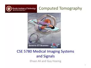
PAM2003Lecture 5: Computed Tomography II Image Processing
In this lecture • Briefly re-cap last week’s CT lecture • Image Processing • Back projection • CT or Houndfields numbers • Multiplanar Reformatting (MPR) • Volume Rendering • Partial Volume Effect • Resolution Compromise
Last Time • Short comings of conventional radiography • What is CT • Advantage of CT • Applications of CT • Different Generation Scanners • Spiral CT • Multislice spiral CT
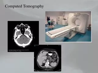
Re-cap • Cross-sectional ‘slices’ • Eliminate superposition
Sheet X-ray beam patient Array of detectors Re-cap: Principles • Use a series of 2D views through an object to calculate its contents • Slice defined by ‘sheet’ of x-rays, produced by a fan beam (typically 1 cm thick) • Thin slice also serves to reduce scatter Rotate tube & detectors through 360º Computer reconstruction of 2D slices
Re-cap: Measurement • Total attenuation between tube & detector • Sum of attenuation coefficients in all voxels beam has travelled through • A measure of how rapidly x-ray are absorbed along line within material • Goal: To calculate attenuation within each individual voxel attenuation
volume element (VOXEL) picture element (PIXEL) slice thickness Re-cap: CT Image • Slice subdivided into matrix of tissue voxels • Voxels correspond to locations in computer memory or pixels in image • Brightness of each pixel governed by x-ray attenuation in corresponding voxel
What We Measure • Detectors measure X-ray intensity after attenuation through patient • Attenuation equal to sum of attenuation in each pixels beam has travelled through • Computer accounts for ‘fan’ shaped beam Total X-ray intensity transmitted through column
Back Projection Simplistic case of sphere in centre of object Simple Analogy • Many projection angles • Detector records total attenuation • Columns filled with total • Overlying projections build up image • More projections increase image quality 8 projections 4 projections 2 projections 64 projections 32 projections 16 projections
Back Projection Simple Arithmetic Example 15 • Simplistic case • 3 X 3 array of pixels 5 5 30 10 10 15 15 5 10 30 30 15 30 10 5 - Sum of all 4 projections ÷
Back Projection Simple Arithmetic Example 15 • Simplistic case • 3 X 3 array of pixels 5 5 30 10 10 15 15 5 10 30 30 15 30 10 5 - 10 Sum of all 4 projections ÷11
Filtered Back Projection • Back projection causes blurring • Compensated by computer using process called ‘filtering’ • Effectively modifies brightness near edge of each back-projected beam Back projected image Filtered back projected image
CT Numbers • Attenuation coefficient of each pixel is compared to that of water, μW • Multiplier (1000) used to obtain whole numbers • Defined as: -1000 for air 0 for water • Varies with kV
+100 Bone +1000 liver window level (WL) muscle blood window width (WW) 0 CT number lung fat Air -1000 -100 Windowing • 2000 CT numbers • Human eye can only perceive ~64 levels • Soft tissue (ex. Fat & lungs) only covers ~80 CT numbers • WL & WW set independently to differentiate different tissues • Pixels with CT numbers outside window are undifferentiated, displayed as black or white
Windowing • Allows differentiation of different tissues WW: 530 WL:-590 WW: 400 WL: -12 • Same image, Different windowing
Multiplanar Reconstruction (MPR) • Data acquired as a series of Axial slices Axial slices
Multiplanar Reconstruction (MPR) • MPR reformats data into Coronal & Sagittal slices Sagittal slices Coronal slices
Partial volume effect • CT cannot reveal detail within voxel • Small high contrast objects raise CT of entire pixel • Tiny calcifications • Traces of contrast media • Reduce effect by using thinner slice
Resolution Compromise • Max spatial and contrast resolution cannot be achieved without unacceptably high dose • E.g. Doubling contrast requires without increasing pixel size requires 4 times increase in dose
Summary • Image Processing • Back projection • CT or Houndfields numbers • Multiplanar Reformatting (MPR) • Volume Rendering • Partial Volume Effect • Resolution Compromise