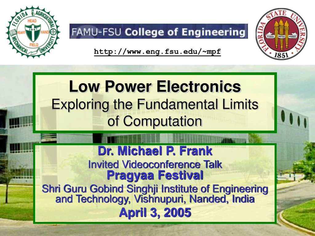
Low Power Electronics Exploring the Fundamental Limits of Computation

1. http://www.eng.fsu.edu/~mpf Low Power ElectronicsExploring the Fundamental Limits of Computation Dr. Michael P. Frank Invited Videoconference TalkPragyaa Festival Shri Guru Gobind Singhji Institute of Engineering and Technology, Vishnupuri, Nanded, India April 3, 2005

2. Abstract of Talk • The electronics industry is rapidly approaching various fundamental physical limits to the energy efficiency of conventional digital technologies. • As a result, the performance of practical digital systems based on conventional technology must level off within at most 1-3 decades. • Our generation will be forced to deal with the consequences! • There is only one potential way to circumvent all these limits that is consistent with the known laws of physics. • Namely: To develop highly reversible computing technologies. • These recycle and reuse most of the logic signal energy. • Reversible computing opens the door to potentially unlimited future improvements in computer efficiency. • This could have enormous potential implications! • But, to develop reversible computing into a fully practical technology is a very challenging engineering problem… • The world’s brightest, most creative people will be needed to solve it! • With hard work, maybe you will be the one to make the key breakthroughs! M. Frank, "Low-Power Electronics"

3. Computer Performance versus Power • Computer performance Π is defined as the rate at which operations (of some standard size) are performed; • i.e., the number nop of operations per unit t of time, Π ≡ nop/t. • Example: Boolean logic operations per second. • In contrast, power P in physics refers to an amount E of energy per unit of time t, that is, P ≡ E/t. • I.e., a rate at which energy undergoes some process. • E.g., being transmitted, transformed, or dissipated to heat. • The question of exactly what the power/energy is doing is a crucial one! • Please, please! Do not confuse this technical meaning of the word “power” with other, more informal uses in English! • E.g., to mean performance: • “My computer is more powerful than yours.”  You really mean, it has better performance. • Or to mean energy: • “How much power do we require in order to add two numbers?”  You really mean, how much energy must be dissipated. M. Frank, "Low-Power Electronics"

4. Computational Energy Efficiency • We define the energy efficiencyηE of a computer as its performance per unit of organized power being used up, ηE ≡ Π/Pdiss. • Where “used up” means transformed into disorganized waste heat power that is dissipated out into the environment. • Therefore, ηE = (nop/t)/(Ediss/t) = nop/Ediss. • Energy efficiency is thus also the number of operations that can be performed per unit of energy that is dissipated. • High energy efficiency is desirable because it can allow us to: • Compute faster while consuming power at a given fixed level, or… • Perform more computational work before running out of energy. • Let Ediss,op denote the amount of energy dissipated in performing 1 standard operation. • Note this has a reciprocal relationship with energy efficiency. • That is, we have ηE = (1 op)/Ediss,op and Ediss,op = (1 op)/ηE. • Thus, high energy efficiency ηE low Ediss,op. M. Frank, "Low-Power Electronics"

5. Trend of Min. Transistor Switching Energy Based on ITRS ’97-03 roadmaps fJ Node numbers(nm DRAM hp) Practical limit for CMOS? aJ Naïve linear extrapolation zJ M. Frank, "Low-Power Electronics"

6. Lower Bounds on Energy Dissipation • In today’s 90 nm VLSI technology, for minimal operations (conventional switching of a minimum-sized transistor): • Ediss,op is on the order of 1 fJ (femtojoule)  ηE≲ 1015 ops/sec/watt. • Will be a bit better in coming technologies (65 nm, maybe 45 nm) • Conventional digital technologies are subject to several lower bounds on their energy dissipation Ediss,op for digital logic / storage / communication operations, • And thus, corresponding upper bounds on their energy efficiency. • Some of the known bounds include: • Leakage-based limit for high-performance field-effect transistors: • Roughly at least ~5 aJ (attojoules)  ηE≲ 2×1017 operations/sec/watt • Reliability-based limit for all non-energy-recovering technologies: • Roughly 1 eV (electron-volt)  ηE≲ 6×1018 operations/sec/watt • von Neumann-Landauer (VNL) bound for all irreversible technologies: • Exactly kT ln 2 ≈ 18 meV (on Earth)  ηE≲ 3.5×1020 operations/sec/watt M. Frank, "Low-Power Electronics"

7. Reliability Bound on Logic Signal Energies • Let Esig denote the logic signal energy, • The energy involved in storing, transmitting, or transforming a bit’s worth of digital information. • But note that “involved” does not necessarily mean “dissipated!” • As a result of fundamental thermodynamic considerations, it is required that Esig ≥ kBTsig ln R, • Where kB is Boltzmann’s constant, 1.38×10−12 J/K; • Tsig is the temperature of the local subsystem carrying the signal; • R is the reliability factor, i.e., the improbability 1/perr of error. • In non-energy-recovering logic technologies (totally dominant today) • Basically all of the signal energy (and often additional energy) is dissipated to heat on each operation. • In this case, minimum sustainable dissipation is Ediss,op≳ kBTenv ln R • Where Tenv is the temperature of the waste-heat reservoir • Averages around 300 K (room temperature) in Earth’s atmosphere • For a decent R = 2×1017, this energy is ~40 kT ≈ 1 eV. • For better energy efficiency, we mustrecover some of the signal energy. • Rather than dissipating it all to heat with each manipulation of the signal. M. Frank, "Low-Power Electronics"

8. VNL Bound on Energy Dissipation from Information Loss Follows directly from the reversibility of fundamental physics! N physical microstates per logical macrostatebefore bit erasure(shown as 8 for clarity in this simple example) Physicalmicrostatetrajectories Logical state “0”,after operation S = k ln 8 = 3 bits S = k ln 16 = 4 bits Logical state “0”,before operation ∆S = 1 bit= k ln 2 Logical state “1”,before operation Ediss = ∆S·Tenv = kTenv ln 2 S = k ln 8= 3 bits M. Frank, "Low-Power Electronics"

9. Von Neumann-Landauer Bound • Follows directly from the time-reversibility (invertibility) of all fundamental physical dynamics. • This in turn is implied by the Hamiltonian formulation of mechanics; and the unitarity of quantum mechanics.  Very well-established. • Implies that physical information can never be destroyed! • Only reversibly transformed! • When we lose or discard a bit’s worth of logical information, • e.g., by erasing or destructively overwriting a bit storage location… • the ‘lost’ information must actually remain in existence, • if in no other form, then as a bit’s worth (k ln 2) of physical entropy. • Entropy simply means unknown information in the physical state. • If the logical bit was originally known (not entropy) • then entropy has increased in this process by ∆S = 1 bit = k ln 2. • The energy in the heat reservoir must be increased by an amount ∆S·Tenv = kTenv ln 2 in order to contain this additional entropy. M. Frank, "Low-Power Electronics"

10. Reversible Computing • The basic idea is simply this: • Don’t erase information when performing logic / storage / communication operations! • Instead, just reversibly transform it in place! • When reversible digital operations are implemented using well-designed energy-recovering circuitry, • This can result in energy dissipation Ediss << Esig, • This has already been empirically demonstrated in many chips. • and even (in principle) energy dissipation Ediss << kT ln 2! • This is pretty clear in theory, but we are not yet to the point of achieving such low levels of dissipation experimentally. • Achieving this goal requires very careful design, • and verifying it requires very sensitive measurement equipment. M. Frank, "Low-Power Electronics"

11. Adiabatic Circuits • Reversible logic can be implemented today using fairly ordinary voltage-coded CMOS VLSI circuits. • With a few changes to the logic-gate/circuit architecture. • We avoid dissipating most of the circuit node energy when switching, by transferring charges in a nearly adiabatic (literally, “without flow of heat”) fashion. • I.e., asymptotically thermodynamically reversible. • In the limit, as various low-level technology parameters are scaled. • There are many designs for purported “adiabatic” circuits in the literature, • but, watch out! Most of designs out there contain fatal flaws, and are not truly adiabatic. • Many past designers are unaware of (or accidentally failed to meet) all the requirements for true thermodynamic reversibility. M. Frank, "Low-Power Electronics"

12. Reversible and/or Adiabatic VLSI Chips Designed @ MIT, 1996-1999 By Frank and other then-students in the MIT Reversible Computing group,under CS/AI lab members Tom Knight and Norm Margolus.

13. Bistable Potential-Energy Wells A Technology-Independent Model of Digital Devices (Landauer ’61) • Consider any system having an (adjustable) potential energy surface (PES) in its configuration space. • The PES should have at least two local minima (or wells) • Therefore the system is bistable • It has two stable (or at least metastable) configurations • Located at well bottoms • The two stable states form a natural bit. • One state can represent 0, the other 1. • This picture can also be easily generalized tolarger numbers of stable states. • Consider now the PES havingtwo adjustable parameters: • (1) “Height” (energy) of the potential energy barrier between wells, relative to well bottoms • (2) Relative height of the left and rightstates in the well (call this “bias”) Potentialenergy 0 1 Generalizedconfigurationcoordinate

14. Possible Parameter Settings • In some of the following slides, we will mention six qualitatively different settings of the well parameters, as shown below… Raised BarrierHeight Lowered Left Neutral Right Direction of Bias Force

15. MOSFET Implementation • The logical state is in the location of a charge packet (excess of electrons) on either side terminal of a FET. • The charge packet might even consist of just a single excess electron in a sufficiently small (nanoscale) logic node. • The potential energy barrier is provided by the built-in voltage across the PN junctions in the FET. • The barrier height is lowered when the device is turned on by adjusting the voltage on the gate electrode. • Bias forces can be provided by (e.g.) capacitive coupling to nearby electrodes. n p n e e e

16. Possible Well Transitions (Ignoring superposition states.) • Catalog of all the possible transitions in the bistable wells, adiabatic & not... • We can characterize a wide variety of digitallogic and memory styles in terms of how theiroperation corresponds to subgraphs of this diagram. “1”states 1 1 1 leak 0 “0”states 0 leak 0 BarrierHeight ∆E k ln 2 ∆E N 1 0 Direction of Bias Force

17. Ordinary Irreversible Logics • Principle of operation: Lower a barrier, or not, based on input. Series/parallel combinations of barriers do logic. Major dissipation in at least one of the possible transitions. 1 Input changes, barrier lowered • Can amplify input signals. 0 Example: Ordinary CMOS logics Outputirreversiblychanged to 0 0

18. Irreversible SET/CLR operations SET operation • Irreversible SET: Turn on a pFET connecting node B to a high voltage source. B B Voltage color scheme: Low / High ½CV2 B • Irreversible CLR: Turn on an nFET connecting node B to a low voltage source. CLR operation B ½CV2 B B

19. Conventional Logic is Irreversible Even a simple NOT gate, as it’s traditionally implemented! • Here’s what all of today’s logic gates (including NOT) do continually, i.e., every time their input changes: • They overwrite previous output with a function of their input. • Performs many-to-one transformation of local digital state! •  required to dissipate ≳kT on avg., by Landauer principle • Incurs ½CV2 energy dissipation when the output changes. Inverter transition table: Example: Static CMOS Inverter: in out

20. Example: Standard CMOS Inverter Inputgoeshigh Power (Vdd) Power (Vdd) on off In Out In Out = 0 = 0 = 1 = 1 Barrier btwn.Out and Groundlowered, charge“falls” to lowerenergy level off on Inputgoeslow Ground (0V) Ground (0V) Voltage color scheme: Low / High Barrierlowered Barrierraised Barrierlowered Simplified ← picture →of PES Charge falls in Charge falls out Vdd Vdd Out GND Out GND

21. Ordinary Irreversible Memory • (1) Lower a barrier, obliviously erasing stored information.(2) Apply an input bias.(3) Raise the barrier to latch the new informationinto place.(4) Remove inputbias. (4) Retractinput 1 1 (1) and (2) can also be in theopposite order (4) Dissipationhere can bemade as low as kT ln 2 Retractinput 0 Barrierup 0 (3) Barrier up (3) (1) Examples:ordinaryDRAM cell,rod logicregister Input“1” Input“0” N 1 0 (2) (2)

22. Example: NMOS latch / DRAM cell Voltage color scheme: Low / Medium / High • Sequence corresponds exactly to general picture illustrated on previous slide. I M I M I M I M on off off off I M on I M I M I M I M on off off off (2) Apply inputbias (3)Raisebarrier (1) Obliviouserasure (4) Remove inputbias (& backto start) Could also do these in the other order also

23. Conventional charging: Constant voltage source Energy dissipated: Ideal adiabatic charging: Constant current source Energy dissipated: Conventional vs. Adiabatic Charging For charging a capacitive load C through a voltage swing V Note: Adiabatic beats conventional by advantage factor A = t/2RC.

24. Adiabatic Switching with MOSFETs • Use a voltage ramp to approximate an ideal current source. • Switch conditionally,if MOSFET gate voltage Vg > V+VT during ramp. • Can discharge the load later using a similar ramp. • Either through the same path, or a different path.t≫RC t≪RC Exact formula:given speed fractions :RC/t Athas ’96, Tzartzanis ‘98

25. Requirements for True Adiabatic Logicin Voltage-coded, FET-based circuits • Avoid passing current through diodes. • Crossing the “diode drop” leads to irreducible dissipation. • Follow a “dry switching” discipline (in the relay lingo): • Never turn on a transistor when VDS≠ 0. • Never turn off a transistor when IDS ≠ 0. • Together these rules imply: • The logic design must be logically reversible • There is no way to erase information under these rules! • Transitions must be driven by a quasi-trapezoidal waveform • It must be generated resonantly, with high Q • Of course, leakage power must also be kept manageable. • Because of this, the optimal design point will not necessarily use the smallest devices that can ever be manufactured! • Since the smallest devices may have insoluble problems with leakage. Importantbut oftenneglected!

26. Reversible Set (rSET) & Clear (rCLR) • rSET operation semantics: Given assurance that a bit is initially 0,unconditionally change it to 1. • To implement: Traverse the adiabat (reversible trajectory) shown below. • Reverse this path to perform rCLR. (6) “1”states 1 1 Put workback in (1) “0”states 0 0 (5) Get workout BarrierHeight (2) (4) (3) N 1 0 Direction of Bias Force

27. rSET/rCLR transition tables • Note that these tables are not reversible according to the strict traditional definition… • Since they don’t represent a 1-1 transformation of all possible input states. • However, if we restrict our use of these operations so as to always avoid the input states that actually result in dissipation, • Then, we obtain a 1-1 transformation of the subset of the input states that are actually used, • And that is the correct statement of the true logical requirement for avoiding Landauer’s principle!

28. Type 1: Input-Bias Clocked-Barrier Reversible Latching (& Logic) (Can amplify/restore input signalin the barrier-raising step.) • Cycle of operation: • (1)Data input applies bias • Add forces to do majority logic • (2) Clock signal raises barrier • (3) Data input bias removed (3) 1 1 (4) Can reset latch reversibly (4) given copy ofcontents. (3) 0 0 (2) (4) (4) (4) (2) (1) (1) Examples:AdiabaticQCA, SCRL latch, Rod logic latch, PQ logic,Buckled logic, Helical logic N 1 0 (4) (4)

29. Type 1 Example: Adiabatic NMOS latch / DRAM cell • Same as irrev. latch, just skip the erasure step! Voltage color scheme: Low / Medium / High I M I M I M on off off I M on I M I M I M Can similarly use a CMOS transmissiongate (nFET/pFET pair) to latch a full-swing signal if necessary. on off off (1) Apply inputbias (2)Raisebarrier (3) Remove inputbias (Reverse stepsto reversiblyunlatch M)

30. P A Simple Reversible CMOS Latch • Uses a single standard CMOS transmission gate (T-gate). • Sequence of operation:(0) input level initially tied to latch ‘contents’ (output); (1) input changes gradually  output follows closely; (2) latch closes, charge is stored dynamically (node floats); (3) afterwards, the input signal can be removed. Before Input Inputinput: arrived: removed:inoutinoutinout0 0 0 0 0 0 1 1 0 1 P in out • Later, we can reversibly “unlatch” the data with an exactly time-reversed sequence of steps. (0) (1) (2) (3) “Reversible latch”

31. Type 2: Input-Barrier, Clocked-Bias Reversible Retractile Logic • Barrier signal is amplified! Gain, restoring logic, fan-out. • Must reset output prior to changing input. • Combinational logic only! • Cycle of operation: • (1) Inputs raise or lower barriers • Do logic w. series/parallel barriers • (2) Clock applies bias force, which changes state, or not 0 0 0 (1) Input barrier height Examples:Hall’s logic,SCRL gates,Rod logic interlocks N 1 0 (2) Clocked bias force applied 

32. Type 2 example: Adiabatic CMOS “buffer” (really, a cSET/cCLR gate) • Controlled-SET / controlled-CLEAR. • Structure: Essentially just a pair of CMOS transmission gates • 2 transistors each, an nFET and a pFET in parallel • Using dual-rail signaling, we can reversibly set or clear a bit on an unoccupied logic node (pair of voltage nodes), conditionally on an input node. • Amplifies input signal. • Fully restores logic levels. DriveN DriveN InN InN InP InP on on DriveN OutN OutN Voltage color scheme: Low / High DriveN DriveN InN off InN InN InP InP off off InP OutN OutN OutN (And similarly for OutP)

33. Transition Table for cSET • It is not unconditionally reversible, • Not a one-to-one transformation of all possible local states, • But, it isconditionally reversible • I.e., on condition that input state 1,1 is avoided.

34. Type 2 example: SCRL inverter • Same structure as static CMOS inverter, but used reversibly. • Produces a fully-restored, amplified output signal. • Inverters can be cascaded, but need latches to get feedback. driveH driveH off off driveH In Out In Out on on off driveL driveL In Out driveH driveH off on on In Out In Out driveL off off Voltage color scheme: Low / Medium / High driveL driveL

35. SCRL Inverter Transition Table • Conditionally reversible, if input is valid and output is ½ just before drivers do their thing. • No point in even listing the table entries that don’t occur; can summarize operation below.

36. Example: Adiabatic NMOS OR gate • Input barriers along two parallel paths A A Out Out Drive Drive Out = A B B B A A • Reverse sequence decomputes Out. • Can’t change A,B freely until then. • With NMOS, Out is weak (orange). • Can use an SCRL inverter to restore the signal levels. • If appropriately biased… • Or, just use CMOS transmission gates instead (8T OR) Out Out Drive Drive A B B Out Drive A A B Out Out Drive Drive B B A A Out Out Drive Drive B B

37. Type 3: Input-Barrier, Clocked-Bias Latching Logic ● Cycle of operation: • Input conditionally lowers barrier • Do logic w. series/parallel barriers • Clock applies bias force; conditional bit flip • Input removed, raising the barrier &locking in the state-change • Clockbias canretract 1 (4) (4) 0 0 0 (2) (2) (3) (1) Examples:Mike’s4-cycle 2-level adiabaticCMOS logic (2LAL) (2) (2) N 1 0

38. 2LAL: 2-level Adiabatic Logic A pipelined fully-adiabatic logic invented at UF (Spring 2000),implementable using ordinary CMOS transistors. TN T • Use simplified T-gate symbol: • Basic buffer element: • cross-coupled T-gates: • need 8 transistors to buffer 1 dual-rail signal • Only 4 timing signals 0-3 areneeded. Only 4 ticks per cycle: • i rises during tickst≡i (mod 4) • i falls during ticks t≡i+2 (mod 4) 2 : 1 (implicitdual-railencodingeverywhere) in TP out 0 Animation: Tick # 0 1 2 3 … 0 1 2 3

39. 2LAL Cycle of Operation Tick #0 Tick #1 Tick #2 Tick #3 11 in1 in0 10 out1 in 01 00 11 in=0 out0 out=0 01 00

40. 2LAL Shift Register Structure Animation: • 1-tick delay per logic stage: • Logic pulse timing and signal propagation: 1 2 3 0 in@0 out@4 0 1 2 3 0 1 2 3 ... 0 1 2 3 ... inN inP

41. More Complex Logic Functions 0 AND gate (plus delayed A) OR gate • Non-inverting multi-input Boolean functions: • One way to do inverting functions in pipelined logic is to use a quad-rail logic encoding: • To invert, justswap the rails! • Zero-transistor“inverters.” A0  A0 B0 A1 B0 (AB)1 (AB)1 A = 0 A = 1 AN AP AN AP

42. Cadence simulation results Work by AdiaMEMS project students:Krishna NatarajanVenkiteswaran Anantharam(UF ECE Dept., under supervision of Dr. Frank, CISE/ECE)

43. <.01× the power @ 1 MHz >100× faster @ 1 pW/T Simulation Results from Cadence • Assumptions & caveats: • Assumes ideal trapezoidal power/clock waveform. • Minimum-sized devices, 2λ×3λ* .18 µm (L) × .24 µm (W) • nFET data is shown* pFETs data is very similar • Various body biases tried * Higher Vth suppresses leakage • Room temperature operation. • Interconnect parasitics have not yet been included. • Activity factor (transitions per device-cycle) is 1 for CMOS, 0.5 for 2LAL in this graph. • Hardware overhead from fully- adiabatic design style is not yet reflected * ≥2× transistor-tick hardware overhead in known reversible CMOS design styles 1 nJ 100 pJ Standard CMOS 10 pJ 10 aJ 1 pJ 1 aJ 1 eV Energy dissipated per nFET per cycle 100 fJ 2V 100 zJ 2LAL 1.8-2.0V 1V 10 fJ 10 zJ 0.5V 0.25V 1 fJ kT ln 2 1 zJ 100 aJ 100 yJ

44. S A B S A B S A B S A B S A B S A B S A B S A B G Cin GCoutCin GCoutCin G Cin GCoutCin G Cin GCoutCin G Cin P P P P P P P P PmsGlsPls Pms GlsPls PmsGlsPls Pms GlsPls MS MS LS LS G G GCout Cin GCout Cin P P P P Pms GlsPls Pms GlsPls MS LS G GCout Cin P P Pms GlsPls LS GCout Cin P O(log n)-time carry-skip adder With this structure, we can do a2n-bit add in 2(n+1) logic levels→ 4(n+1) reversible ticks→ n+1 clock cycles.Hardwareoverhead is<2× regularripple-carry. (8 bit segment shown) 3rd carry tick 2nd carry tick 4th carry tick 1st carry tick

45. 20x better perf.@ 3 nW/adder 32-bit Adder Simulation Results 1V CMOS 1V CMOS 0.5V CMOS 0.5V CMOS 2V 2LAL, Vsb=1V 2V 2LAL, Vsb=1V (All results normalized to a throughput level of 1 add/cycle)

46. Thanks to AdiaMEMS Project Members Left toRight: Venki,Mike,Maojiao,Krishna, & Huikai M. Frank, "Low-Power Electronics"

47. Power per device, vs. frequency Plenty of room for device improvement… • Recall, irreversible device technology has at most ~3-4 orders of magnitude of power-performance improvements remaining. • And then, the firm kT ln 2 limit is encountered. • But, a wide variety of proposed reversible device technologies have been analyzed by physicists. • With theoretical power-performance up to 10-12 orders of magnitude better than today’s CMOS! • Ultimate limits are unclear. .18µm CMOS .18µm 2LAL k(300 K) ln 2 Variousreversibledevice proposals

48. A Potential Scaling Scenario for Reversible Computing Technology • Assume energy coefficient (energy diss. / freq.) of reversible technology continues declining at historical rate of 16× / 3 years, through 2020. • For adiabatic CMOS, cE = CV2RC = C2V2R. • This has been going as ~4 under constant-field scaling. • Requires new devices after CMOS scaling stops. • But, many potential candidates are waiting in the wings… • Assume affordable number of layers of active circuitry per chip (or per package, e.g., stacked dies) doubles every 3 years, through 2020. • Competitive pressures will tend to reduce per-layer cost, esp. if device-size scaling stops, as assumed.

49. Result of Scenario 40 layers, ea. w.8 billion activedevices,freq. 180 GHz,0.4 kT dissip.per device-op e.g. 1 billion devices actively switching at3.3 GHz, ~7,000 kT dissip. per device-op Note that by 2020, there could be a factor of 20,000× difference in rawperformance per 100W package. (E.g., a 100× overhead factor from reversible design could be absorbed while still showing a 200× boost in performance!)

50. Possible Cosmic (!) Implications of Reversible Computing • Astrophysicists Krauss and Starkman have argued that, • even if we someday colonize the stars, • The total energy we can ever harvest is finite! • We can never reach galaxies beyond a certain distance, • due to the accelerating expansion of the universe. • Thus if we never create reversible computing, • Then someday we must run out of energy! (Due to VNL.) • And then, all computation (thus all life) will permanently cease. • However, if we invent reversible computing, • and if we can make it ever more energy-efficient over time, • Then potentially, an infinite number of computations (thoughts?) can be performed using only a finite supply of energy! •  Reversible computing is needed to save the universe! • If Krauss & Starkman’s basic arguments are correct. M. Frank, "Low-Power Electronics"