1 / 63

Computation of Fundamental matrix F

Computation of Fundamental matrix F. Basic equations. x’ T F x = 0 x’= ( x’, y’, 1) T x = ( x, y, 1) T. Basic equations 2. Basic equations 2. The singularity constraint. The singularity constraint 2. The singularity constraint 3. Fig. 10.1 Epipolar lines.

avak
Download Presentation

Computation of Fundamental matrix F

An Image/Link below is provided (as is) to download presentation Download Policy: Content on the Website is provided to you AS IS for your information and personal use and may not be sold / licensed / shared on other websites without getting consent from its author. Content is provided to you AS IS for your information and personal use only. Download presentation by click this link. While downloading, if for some reason you are not able to download a presentation, the publisher may have deleted the file from their server. During download, if you can't get a presentation, the file might be deleted by the publisher.

E N D

Presentation Transcript


  1. Computation of Fundamental matrix F

  2. Basic equations • x’T F x = 0 • x’= (x’, y’, 1)T x = (x, y, 1)T

  3. Basic equations 2

  4. Basic equations 2

  5. The singularity constraint

  6. The singularity constraint 2

  7. The singularity constraint 3

  8. Fig. 10.1 Epipolar lines

  9. Epipolar lines

  10. 10.2 The normalized 8 point algorithm

  11. The normalized 8 point algorithm

  12. The normalized 8 point algorithm

  13. Computing F: Recommendations

  14. Image pairs with epipoles far from the image centres Fig 10.2

  15. Image pairs with epipoles close to the image centres Fig. 10.2

  16. Automatic computation of F

  17. Automatic computation of F 2

  18. Automatic computation of F 3

  19. Automatic computation of fundamental matrix using RANSAC 640 x 480 pixels

  20. Detected corners(500) superimposed on the images

  21. 188 putative matches shown by the line linking corners, 89 are outliers

  22. Inliners –99 correspondences consistent with the estimated F

  23. Final set of 157 correspondence after guided matching using MLE, with a few mismatches(e.g. the long line on the left)

  24. Special cases of F-computation

  25. Fig. 10.5 for a pure translation, the epipole can be estimated from the image motion of two points

  26. Translational motion

  27. 10. 7.2 Planar motion

  28. 10.7.3 The calibrated case

  29. 10.7.3 The calibrated case 2

  30. 10.8 Correspondence of other entitiesLine 1

  31. 10.8 Correspondence of other entitiesLine 2

  32. 10.8 Correspondence of other entitiesSpace curves

  33. 10.8 Correspondence of other entitiesSurfaces

  34. Epipolar tangency

  35. Fig.10.6 Epipolar tangency

  36. 10.9 Degeneracies

  37. Table 10.1

  38. 10.9.1 Points on a ruled quadric

  39. 10.9.1 Points on a ruled quadric 2

  40. 10.9.2 Points on a plane

  41. 10.9.2 Points on a plane 2

  42. 10.9.2 Points on a plane 3

  43. 10.9.3 No translation:The epipolar geometry is not defined.Two images are related by a 2D homography

  44. 10.12 Image rectification

  45. 10.12 Image rectification 2

  46. Mapping the epipole to infinity

  47. Force the transformation H to be rigid transformation in the neighborhood of x0A good choice of x0 be the image centre

  48. X0 is the origin

  49. X0 is arbitrary placed point of interest

More Related