Download
1 / 26
260 likes | 332 Views
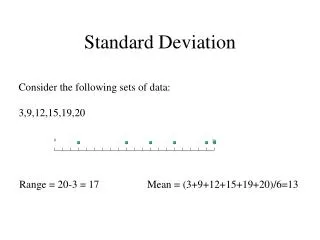
Standard Deviation. Lecture 18 Sec. 5.3.4 Tue, Feb 15, 2005. 0. 1. 2. 3. 5. 6. 7. 8. x = 4. Deviations from the Mean. Each unit of a sample or population deviates from the mean by a certain amount. Define the deviation of x to be ( x – x ). 0. 1. 2. 3. 5. 6. 7. 8.

E N D
Standard Deviation Lecture 18 Sec. 5.3.4 Tue, Feb 15, 2005
0 1 2 3 5 6 7 8 x = 4 Deviations from the Mean • Each unit of a sample or population deviates from the mean by a certain amount. • Define the deviation of x to be (x –x).
0 1 2 3 5 6 7 8 x = 4 Deviations from the Mean • Each unit of a sample or population deviates from the mean by a certain amount. deviation = –4
0 1 2 3 5 6 7 8 x = 4 Deviations from the Mean • Each unit of a sample or population deviates from the mean by a certain amount. dev = 1
0 1 2 3 5 6 7 8 x = 4 Deviations from the Mean • Each unit of a sample or population deviates from the mean by a certain amount. deviation = 3
Sum of Squared Deviations • We want to add up all the deviations, but to keep the negative ones from canceling the positive ones, we square them all first. • So we compute the sum of the squared deviations, called SSX. • Procedure • Find the deviations • Square them all • Add them up
Sum of Squared Deviations • SSX = sum of squared deviations • For example, if the sample is {0, 5, 7}, then SSX = (0 – 4)2 + (5 – 4)2 + (7 – 4)2 = (-4)2 + (1)2 + (3)2 = 16 + 1 + 9 = 26.
The Population Variance • Variance of the population – The average squared deviation for the population. • The population variance is denoted by 2.
The Sample Variance • Variance of a sample – The average squared deviation for the sample, except that we divide by n – 1 instead of n. • The sample variance is denoted by s2. • This formula for s2 makes a better estimator of 2 than if we had divided by n.
Example • In the example, SSX = 26. • Therefore, s2 = 26/2 = 13.
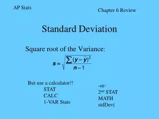
The Standard Deviation • Standard deviation – The square root of the variance of the sample or population. • The standard deviation of the population is denoted . • The standard deviation of a sample is denoted s.
Example • In our example, we found that s2 = 13. • Therefore, s = 13 = 3.606.
Example • Example 5.10, p. 293. • Use Excel to compute the mean and standard deviation of the height and weight data. • HeightWeight.xls. • Use basic operations. • Use special functions.
Alternate Formula for the Standard Deviation • An alternate way to compute SSXis to compute • Note that only the second term is divided by n. • Then, as before
Example • Let the sample be {0, 5, 7}. • Then x = 12 and x2 = 0 + 25 + 49 = 74. • So SSX = 74 – (12)2/3 = 74 – 48 = 26, as before.
TI-83 – Standard Deviations • Follow the procedure for computing the mean. • The display shows Sx and x. • Sx is the sample standard deviation. • x is the population standard deviation. • Using the data of the previous example, we have • Sx = 3.605551275. • x = 2.943920289.
Interpreting the Standard Deviation • Both the standard deviation and the variance are measures of variation in a sample or population. • The standard deviation is measured in the same units as the measurements in the sample. • Therefore, the standard deviation is directly comparable to actual deviations.
Interpreting the Standard Deviation • The variance is not comparable to deviations. • The most basic interpretation of the standard deviation is that it is roughly the average deviation.
Interpreting the Standard Deviation • Observations that deviate fromx by much more than s are unusually far from the mean. • Observations that deviate fromx by much less than s are unusually close to the mean.
Interpreting the Standard Deviation s s x – s x x + s
Interpreting the Standard Deviation Closer than normal tox x – s x x + s
Interpreting the Standard Deviation Farther than normal fromx x – s x x + s
Interpreting the Standard Deviation Unusually far fromx x – 2s x – s x x + s x + 2s
Let’s Do It! • Let’s do it! 5.13, p. 295 – Increasing Spread. • Let’s do it! 5.14, p. 297 – Variation in Scores.