Download
1 / 19
200 likes | 418 Views
Compressive sampling and dynamic mode decomposition. Steven L. Brunton1, Joshua L. Proctor2, J. Nathan Kutz1 , Journal of Computational Dynamics, Submitted in DEC,2013. Dynamic Mode Decomposition. Motivation.

E N D
Compressive sampling and dynamic mode decomposition Steven L. Brunton1, Joshua L. Proctor2, J. Nathan Kutz1, Journal of Computational Dynamics, Submitted in DEC,2013.
Dynamic Mode Decomposition • Motivation • Fluid simulation is very important in engineering. in that most fluid mechanical systems of interest are described by the same governing equations: the Navier–Stokes equations. • Unfortunately, the Navier–Stokes equations are a set of nonlinear partial differential equations that give rise to all manner of dynamics, including those characterized by bifurcations, limit cycles, resonances, and full-blown turbulence. In some cases, It’s difficult to find analytic solutions. This forces people to rely on experiments and high-performance computations when studying such systems.
Dynamic Mode Decomposition • Motivation • As experiments and computations become more advanced, they generate ever increasing amounts of data. Manipulating such data to find anything but the most obvious trends requires a skillset all its own. This has led to a growing need for data-driven methods that can take a dataset and characterize it in meaningful ways with minimal guidance.
Dynamic Mode Decomposition • Definition • Many in fluid mechanics have turned to modal decomposition as the tool of choice for data-driven analysis. It is a powerful new technique introduced in the fluid dynamics community to isolate spatially coherent modes that oscillate at a fixed frequency. • Generally, a modal decomposition takes a set of data and from it computes a set of modes, or characteristic features. The meaning of the modes depends on the particular type of decomposition used. However, in all cases, the hope is that the modes identify features of the data that elucidate the underlying physics.
Dynamic Mode Decomposition • Difference between traditional methods • DMD is a modal decomposition developed specifically for analyzing the dynamics of nonlinearly evolving fluid flows. It was first introduced in 2008. • Proper orthogonal decomposition (POD), perhaps the most common modal decomposition in the fluids community. but the POD modes are not necessarily optimal for modeling those dynamics. For instance, when analyzing a time-series, the POD modes remain unchanged if the data are reordered; the modes do not depend on the time evolution/dynamics encoded in the data.
Dynamic Mode Decomposition • features of DMD • The DMD is a data-driven and equation-free method that applies equally well to data from experiments or simulations. An underlying principle is that even if the data is high-dimensional, it may be described by a low dimensional attractor subspace defined by a few coherent structures. • DMD not only provides modes, but also a linear model for how the modes evolve n time.
Compressive Sampling and DMD • Main contribution • This Paper deviates from the prior studies combining compressive sampling and DMD, in that we utilize sparsity of the spatial coherent structures to reconstruct full-state DMD modes from few measurements. The resulting DMD eigenvalues are equal to DMD eigenvalues from the full-state data. It is then possible to reconstruct full-state DMD eigenvectors using l1 minimization.
Compute DMD Consider the following data snapshot matrices:
Compressive sampling • The theory of compressive sampling suggests that instead of measuring the high-dimensional signal x and then compressing, it is possible to measure a low-dimensional subsample or random projection of the data and then directly solve for the few non-zero coefficients in the transform basis. C is the measurement matrix. If x is sparse, then we would like to solve the underdetermined system of equations
Compressive DMD • This paper establish basic connections between the DMD on full-state and projected data. These connections facilitate the two main applied results of this work: • It is possible to compute DMD on projected data and reconstruct full-state DMD modes through compressive sampling • If full-state measurements are available, it is advantageous to compress the data, compute the projected DMD, and then compute full-state DMD modes by linearly combining snapshots according to the projected DMD transforms.
Compressive DMD Invariance of DMD to unitary transformations
Compressive DMD Various approaches and algorithms Compressed DMD Compressive sampling DMD
Experiments Double gyre flow
Experiments Double gyre flow
Experiments Double gyre flow
Experiments Flow around a cylinder
Experiments Flow around a cylinder