Download
1 / 34
340 likes | 355 Views
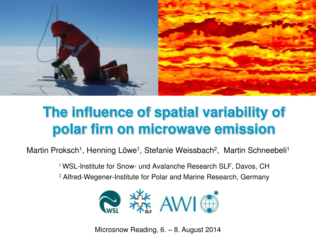
The influence of spatial variability of polar firn on microwave emission. 1 WSL-Institute for Snow- und Avalanche Research SLF, Davos, CH. Martin Proksch 1 , Henning Löwe 1 , Stefanie Weissbach 2 , Martin Schneebeli 1. 2 Alfred-Wegener-Institute for Polar and Marine Research, Germany.

E N D
The influence of spatial variability of polar firn on microwave emission • 1 WSL-Institute for Snow- und Avalanche Research SLF, Davos, CH Martin Proksch1, Henning Löwe1, Stefanie Weissbach2, Martin Schneebeli1 • 2Alfred-Wegener-Institute for Polar and Marine Research, Germany • Microsnow Reading, 6. – 8. August 2014
Outline • Motivation • Instrument and measurements • Simulations and Results • Spatial variability • Layer thickness • Conclusions WSL-Institut für Schnee- und Lawinenforschung SLF
1. Motivation I • Microwave observations are essential in polar regions (think about polar night!) • To understand the microwave signatures of polar firn, in-situ data is necessary, but traditional snow measurements are: • limited in spatial resolution • limited by extensive measurement times • constrained due to harsh polar environments • subjective (variability between observers) • Desirable: fast derivation of the relevant objective parameters with sufficient resolution (e.g. Correlation length and density to model microwave emission) WSL-Institut für Schnee- und Lawinenforschung SLF
1. Motivation II • Where to measure (Sampling design)? • Answer requires knowledge about snow variability! Pic: Martin Schneebeli WSL-Institut für Schnee- und Lawinenforschung SLF
2.1 Instrument: SnowMicroPen (SMP) • Specifications: • High resolution: vertical ~1mm • Fast: 1 m profile ~ 1 minute • Portable => Ideal for spatial variability • Output: • Density, SSA and Correlation length (Proksch et al, submitted) • 2D stratigraphy from transects
2.2 Measurements at Kohnen Station: Density 92 SMP profiles with interval 0.5 m -> 45m transect: WSL-Institut für Schnee- und Lawinenforschung SLF
2.2 Measurements at Kohnen Station: Correlation length lex 92 SMP profiles with interval 0.5 m -> 45m transect: WSL-Institut für Schnee- und Lawinenforschung SLF
2.2 Measurements at Kohnen Station: specific surface area SSA 92 SMP profiles with interval 0.5 m -> 45m transect: WSL-Institut für Schnee- und Lawinenforschung SLF
3.1 MEMLS simulations MEMLS: Microwave Emission Model ofLayeredSnowpacks, Wiesmann andMätzler, 1999. -> withImproved Born Approximation, Mätzler 1998. MEMLS input: • 1cm layerthickness in top mostmeter • lex: SMP (no «grainsize» scaling) • Density: SMP • Snow temperatureprofile • Tsky: 0K • Snow-groundreflectivity: 0 • 20m deepprofile, linearlyincreasing WSL-Institut für Schnee- und Lawinenforschung SLF
3.2 Results: Brightnesstemperatures σ Tb Tb WSL-Institut für Schnee- und Lawinenforschung SLF
3.2 Results: Brightnesstemperatures σ Tb Tb WSL-Institut für Schnee- und Lawinenforschung SLF
3.2 Results: Brightnesstemperatures • One MEMLS run per SMP profile, total N = 92 • σ(Tb, 36GHz) = 16.6 K σ Tb Tb WSL-Institut für Schnee- und Lawinenforschung SLF WSL-Institut für Schnee- und Lawinenforschung SLF 14
3.2 Results: Brightnesstemperatures • One MEMLS run per SMP profile, total N = 92 • σ(Tb, 36GHz) = 16.6 K • Todecreaseσ, wehavetoincreasethenumberofmeasurements N: • σ(Tb) = 16 K • for N=92 • σ(Tb) = 8K • for N = 368 • σ(Tb) = 2K • for N = 2944 σ Tb Tb WSL-Institut für Schnee- und Lawinenforschung SLF
3.2 Results: Summit Standard deviations: • T19GHz, V-pol = 13.9 K • T36GHz, V-pol = 24.1 K • T89GHz, V-pol = 23.5 K Constant Density: Constant corr. length • T19GHz, V-pol = 13.5 K T19GHz, V-pol = 3.7 K T36GHz, V-pol = 26.1 K T36GHz, V-pol = 3.8 K T89GHz, V-pol = 27.8 K T89GHz, V-pol = 7.0 K
3.2 Results: Point Barnola Standard deviations: • T19GHz, V-pol = 3.3 K • T36GHz, V-pol = 11.0 K • T89GHz, V-pol = 21.2 K Constant Density: Constant corr. length • T19GHz, V-pol = 4.5 K T19GHz, V-pol = 1.2 K T36GHz, V-pol = 12.8 K T36GHz, V-pol = 1.5 K T89GHz, V-pol = 23.7 K T89GHz, V-pol = 4.3 K WSL-Institut für Schnee- und Lawinenforschung SLF
3.3 Results: Spatialcorrelations WSL-Institut für Schnee- und Lawinenforschung SLF
3.3 Results: Spatialcorrelations WSL-Institut für Schnee- und Lawinenforschung SLF
3.3 Results: Spatialcorrelations WSL-Institut für Schnee- und Lawinenforschung SLF
3.3 Results: Spatialcorrelations WSL-Institut für Schnee- und Lawinenforschung SLF
3.3 Results: Spatialcorrelations WSL-Institut für Schnee- und Lawinenforschung SLF
3.3 Results: Spatialcorrelations WSL-Institut für Schnee- und Lawinenforschung SLF
3.3 Results: Spatialcorrelations WSL-Institut für Schnee- und Lawinenforschung SLF
3.4 Results: Layer thickness • 20m deep profile: • First meter SMP measurement • 2 – 20 meter: linear increasing, with random noise added. 20 cm 3 cm WSL-Institut für Schnee- und Lawinenforschung SLF
3.4 Results: Effectofverticalaveraging Averaging to 3cm layer thickness leads to significant loss of density variations! WSL-Institut für Schnee- und Lawinenforschung SLF
4. Summary and Conclusions • The SnowMicroPen allows the measurement of full-meter profiles in less than one minute • Transects reveals the 2D quantitative stratigraphy of polar firn • One single profile is not enough – statistically based sampling design? • Layer thickness critical • Outlook: optimize deep profiles to match Satellite data WSL-Institut für Schnee- und Lawinenforschung SLF
s Thankyou! • Thanksto: • Christian Mätzler • Ludovic Brucker WSL-Institut für Schnee- und Lawinenforschung SLF
3.5 Results: Measurement accuracy • Meas. accuracy in top most meter • To model Tb within 1K WSL-Institut für Schnee- und Lawinenforschung SLF
Outlook • Compareto SSMI WSL Institute for Snow and Avalanche Research SLF
To do: • Spat var - forotherstations • Layer thickness • Measaccuracy WSL Institute for Snow and Avalanche Research SLF
3.2 Results: Spatialcorrelations WSL-Institut für Schnee- und Lawinenforschung SLF
3.2 Results: Spatialcorrelations WSL-Institut für Schnee- und Lawinenforschung SLF
3.2 Results: Spatialcorrelations WSL-Institut für Schnee- und Lawinenforschung SLF