Download
1 / 35
350 likes | 448 Views
The sea-breeze circulation. Part II: Effect of Earth ’ s rotation. Reference: Rotunno (1983, J. Atmos. Sci. ). Rotunno (1983). Quasi-2D analytic linear model Heating function specified over land Becomes cooling function after sunset Cross-shore flow u , along-shore v

E N D
The sea-breeze circulation Part II: Effect of Earth’s rotation Reference: Rotunno (1983, J. Atmos. Sci.)
Rotunno (1983) • Quasi-2D analytic linear model • Heating function specified over land • Becomes cooling function after sunset • Cross-shore flow u, along-shore v • Two crucial frequencies • Heating Ω= = 2/day (period 24h) • Coriolisf=2 ω sin(λ) (inertial period 17h @ 45˚N) • One special latitude… where f = (30˚N)
Circulation C Integrate CCW as shown Take w ~ 0; utop ~ 0 Integrate from ±infinity, from sfc to top of atmosphere
Rotunno chooses, w(x,0,t)=0, Fx=0, Fy=0, and defines the heating function Q analytically. Its time dependence is assumed to be the daily periodic signal Q The equations can be written in terms of ψ, following the following steps: - Take time derivative of Eq 1 and call the result Eq 6 - Use Eq. 2 to eliminate v from Eq 6, and call the result Eq 7 - Take the partial with respect to z of Eq 7 and call it Eq 8 - Take time derivative of Eq 3 and call the result Eq 9 - Use Eq. 4 to eliminate b from Eq 9, and call the result Eq 10 - Take the partial with respect to x of Eq 10 and call it Eq 11 - Take the difference between equations 8 and 11
Rotunno’s analytic solution If f >w (poleward of 30˚) equation is elliptic • sea-breeze circulation spatially confined • circulation in phase with heating • circulation, onshore flow strongest at noon • circulation amplitude decreases poleward If f <w (equatorward of 30˚) equation is hyperbolic • sea-breeze circulation is extensive • circulation, heating out of phase • f = 0 onshore flow strongest at sunset • f = 0 circulation strongest at midnight
Rotunno’s analytic solution If f =w (30˚N) equation is singular • some friction or diffusion is needed • circulation max at sunset • onshore flow strongest at noon
Heating function Rotunno’s analytic model lacks diffusion so horizontal, vertical spreading built into function
f >w (poleward of 30˚) at noon Note onshore flow strongest at coastline (x = 0); this is day’s max coast
f <w (equatorward of 30˚) y at three times sunrise noon (reverse sign for midnight) sunset Note coastline onshore flow max at sunset
Max |C| noon & midnight Paradox? • Why is onshore max wind at sunset and circulation max at midnight/noon? • While wind speed at coast strongest at sunset/sunrise, wind integrated along surface larger at midnight/noon
In order to treat the case f=ω (30 degrees) effects of linear friction are included (α is the linear friction parameter)Fx= -α u Fy = -α v Fz =0 Q=H(x,z) sin(ωt) – α b Time of circulation maximum 180 deg midnight 90 deg sunset 0 deg noon friction coefficient As friction increases, tropical circulation max becomes earlier, poleward circulation max becomes later
Dynamics and Thermodynamics Demonstration Model (DTDM): The DTDM is a simple, two-dimensional, script-driven package that can be used to demonstrate concepts relating to: gravity waves produced by heat and momentum sources sea-breeze circulations generated by differential heating lifting over cold pools Kelvin-Helmholtz instability The entire package, was written by Rob Fovell in Fortran 77 and producesGrADSoutput DTDM has been tested on Linux, Mac OS X and other Unix or Unix-like systems, and MS Windows with the g77, g95, IBM (xlf), Portland Group (pgf77) and Intel (ifort) Fortran compilers. http://www.atmos.ucla.edu/~fovell/DTDM/ The Grid Analysis and Display System (GrADS) is an interactive desktop tool that is used for easy access, manipulation, and visualization of earth science data. http://grads.iges.org/grads/head.html
Before going into the details on how to run the program a few considerations on the numerical scheme. In Chapter 6 Fovell summarizes the equations in 2-dimensions without Coriolis NOTE: The final form of the equations going into DTDM, including diffusion and moisture are in Fovell’s notes 8.13-8.19. The Coriolis terms must still be added
There are a variety of approaches to discretization each with different numerical problems. DTDM uses the leapfrog scheme in which space and time derivatives are replaced with centered approximations. For the heat equations (hyperbolic PDE) + c =0
Sound Waves are always present but it can be shown that they imperil the efficient solution of the equations. The need to maintain stability places limits on how large we can choose the model time step to be. For the leapfrog scheme the time step (grid spacing/ speed) is limited by the speed of the fastest moving signal in the model. So for cases with sound speed of ~300 m/s, the great computational expense is caused by the least important aspect of the physical model.
Techniques: Adopt time splitting in which acoustically active and inactive parts are Identified and are solved with different time steps. Relatively economical but difficult to implement 2) Quasi-compressible approach. Artificially slow down the sound waves by treating the sound speed as a free parameter and discounting it. Efficient and easy to code but does violence to the model physics 3) Anaelastic Approximation. Consists on artificially speeding up the waves all the way to infinity. Eliminates the wave contribution and leads to a simple continuity equation It is difficult to implement.
DTDM long-term sea-breeze strategy • Incorporate Rotunno’s heat source, mimicking effect of surface heating + vertical mixing • Make model linear • Dramatically reduce vertical diffusion • Simulations start at sunrise • One use: to investigate effect of latitude and/or linearity on onshore flow, timing and circulation strength
The choices for a particular run are determined in the input control files. Example: input_seabreeze.txt&rotunno_seabreezesection c=================================================================== c c The rotunno_seabreezenamelist implements a lower tropospheric c heat source following Rotunno (1983), useful for long-term c integrations of the sea-land-breeze circulation c c iseabreeze (1 = turn Rotunno heat source on; default is 0) c sb_ampl - amplitude of heat source (K/s; default = 0.000175) c sb_x0 - controls heat source shape at coastline (m; default = 1000.) c sb_z0 - controls heat source shape at coastline (m; default = 1000.) c sb_period - period of heating, in days (default = 1.0) c sb_latitude - latitude for experiment (degrees; default = 60.) c sb_linear (1 = linearize model; default = 1) c c===================================================================
input_seabreeze.txt&rotunno_seabreezesection &rotunno_seabreeze iseabreeze = 1, sb_ampl = 0.000175, sb_x0 = 1000., sb_z0 = 1000., sb_period = 1.0, sb_latitude = 30., sb_linear = 1, $ sb_latitude ≠ 0 activates Coriolis sb_linear = 1 linearizes the model Other settings include: timend = 86400 sec dx = 2000 m, dz = 250 m, dt = 1 sec dkx = dkz = 5 m2/s (since linear)
input_seabreeze.txt&rotunno_seabreezesection &rotunno_seabreeze iseabreeze = 1, sb_ampl = 0.000175, sb_x0 = 1000., sb_z0 = 1000., sb_period = 1.0, sb_latitude = 30., sb_linear = 1, $ sb_latitude ≠ 0 activates Coriolis sb_linear = 1 linearizes the model Other settings include: timend = 86400 sec dx = 2000 m, dz = 250 m, dt = 1 sec dkx = dkz = 5 m2/s (since linear)
Caution • Don’t make model anelastic for now • Make sure ianelastic = 0 and ipressure = 0 • Didn’t finish the code for anelastic linear model • iseabreeze = 1 should be used alone (I.e., no thermal, surface flux, etc., activated)
Heat source sb_hsrc set mproj off set lev 0 4 set lon 160 240 [or set x 80 120] d sb_hsrc