Download
1 / 38
380 likes | 581 Views
The sea-breeze circulation. Part II: Effect of Earth ’ s rotation. Reference: Rotunno (1983, J. Atmos. Sci. ). Rotunno (1983). Quasi-2D analytic linear model Heating function specified over land Becomes cooling function after sunset Equinox conditions Cross-shore flow u , along-shore v

E N D
The sea-breeze circulation Part II: Effect of Earth’s rotation Reference: Rotunno (1983, J. Atmos. Sci.)
Rotunno (1983) • Quasi-2D analytic linear model • Heating function specified over land • Becomes cooling function after sunset • Equinox conditions • Cross-shore flow u, along-shore v • Two crucial frequencies • Heating = 2/day (period 24h) • Coriolis f = 2sin (inertial period 17h @ 45˚N) • One special latitude… where f = (30˚N)
Heating function Rotunno’s analytic model lacks diffusion so horizontal, vertical spreading built into function
Circulation C Integrate CCW as shown Take w ~ 0; utop ~ 0 Integrate from ±infinity, from sfc to top of atmosphere
Rotunno’s analytic solution If f >w (poleward of 30˚) equation is elliptic • sea-breeze circulation spatially confined • circulation in phase with heating • circulation, onshore flow strongest at noon • circulation amplitude decreases poleward If f <w (equatorward of 30˚) equation is hyperbolic • sea-breeze circulation is extensive • circulation, heating out of phase • f = 0 onshore flow strongest at sunset • f = 0 circulation strongest at midnight
Rotunno’s analytic solution If f =w (30˚N) equation is singular • some friction or diffusion is needed • circulation max at sunset • onshore flow strongest at noon
f >w (poleward of 30˚) at noon Note onshore flow strongest at coastline (x = 0); this is day’s max coast
f <w (equatorward of 30˚) y at three times sunrise noon (reverse sign for midnight) sunset Note coastline onshore flow max at sunset
Max |C| noon & midnight Paradox? • Why is onshore max wind at sunset and circulation max at midnight/noon? • While wind speed at coast strongest at sunset/sunrise, wind integrated along surface larger at midnight/noon
Effect of linear friction Time of circulation maximum midnight sunset noon friction coefficient As friction increases, tropical circulation max becomes earlier, poleward circulation max becomes later
DTDM long-term sea-breeze strategy • Incorporate Rotunno’s heat source, mimicking effect of surface heating + vertical mixing • Make model linear • Dramatically reduce vertical diffusion • Simulations start at sunrise • One use: to investigate effect of latitude and/or linearity on onshore flow, timing and circulation strength
input_seabreeze.txt&rotunno_seabreezesection c=================================================================== c c The rotunno_seabreeze namelist implements a lower tropospheric c heat source following Rotunno (1983), useful for long-term c integrations of the sea-land-breeze circulation c c iseabreeze (1 = turn Rotunno heat source on; default is 0) c sb_ampl - amplitude of heat source (K/s; default = 0.000175) c sb_x0 - controls heat source shape at coastline (m; default = 1000.) c sb_z0 - controls heat source shape at coastline (m; default = 1000.) c sb_period - period of heating, in days (default = 1.0) c sb_latitude - latitude for experiment (degrees; default = 60.) c sb_linear (1 = linearize model; default = 1) c c===================================================================
input_seabreeze.txt&rotunno_seabreezesection &rotunno_seabreeze iseabreeze = 1, sb_ampl = 0.000175, sb_x0 = 1000., sb_z0 = 1000., sb_period = 1.0, sb_latitude = 30., sb_linear = 1, $ sb_latitude ≠ 0 activates Coriolis sb_linear = 1 linearizes the model Other settings include: timend = 86400 sec dx = 2000 m, dz = 250 m, dt = 1 sec dkx = dkz = 5 m2/s (since linear)
Caution • Don’t make model anelastic for now • Make sure ianelastic = 0 and ipressure = 0 • Didn’t finish the code for anelastic linear model • iseabreeze = 1 should be used alone (I.e., no thermal, surface flux, etc., activated)
Solution strategy • Model starts at sunrise (6 am) • Equinox presumed (sunset 6 pm) • Heating max at noon, zero at sunset • Cooling at night, absolute max at midnight
Heat source sb_hsrc set mproj off set lev 0 4 set lon 160 240 [or set x 80 120] d sb_hsrc
Time series using GrADS > open seabreeze.rotunno.30deg > set t 1 289 > set z 1 > set x 100 > set vrange -0.0003 0.0003 > set xaxis 0 24 3 > d sb_hsrc > draw xlab hour > draw ylab heating function at surface > draw title heating function vs. time
30˚N linear case (5 m2/s diffusion) seabreeze.gs Shaded: vertical velocity; contoured: cross-shore velocity
30˚N linear case Circulation max @ Sunset Note non-zero C @ 24h… should run several days to spin-up set t 1 289 set z 1 set xaxis 0 24 3 d sum(u,x=1,x=199)
30˚N linear case sunset Onshore flow max ~ 4pm Note non-calm wind @ 24h… should run several days to spin-up
Cross-shore flow and vertical motion at noon (on 1st day) (seabreeze.gs) set t 72
Cross-shore flow and vertical motion at midnight (on 1st day)
Circulation vs. time • Circ magnitude decreases w/ latitude (expected) • 30N circ max at sunset (expected) • Poleward circ max later than expected (noon) • Equator circ max earlier than expected (midnite) • Consistent w/ existence of some friction? midnight Eq 30N 60N 90N sunset
Recall: linear friction effect Time of circulation maximum midnight sunset noon friction coefficient As friction increases, tropical circulation max shifts earlier, poleward circulation max becomes later
t(h after sunrise) x (across-coast) Hovmoller diagrams (seabreeze_hov.gs) What is missing?
Questions to ponder • Why is the onshore flow at 30N strongest in midafternoon? (Heating max was noon) • Why does onshore max occur earlier at 60N? • Why does onshore flow magnitude decrease poleward? • Why does friction shift circulation max time? • Note no offshore flow at equator at all. Why? • How does linear assumption affect results?
Further exploration • Run model longer… how long until statistically steady? • Make model nonlinear • Compare to data • Collect surface data along N-S coastline • Compare to “data” from more sophisticated model
Tips for nonlinear runs • Set sb_linear = 0 • Increase dkx, dkz to avoid computational instability • Example with dkx = 500, dkz = 50 m2/s (probably excessive)
Cross-shore wind at coastlinelinear vs. nonlinear Why are they different?