Download

1 / 94
990 likes | 1.33k Views
Linear Algebra. 國立勤益科技大學. National Chin-Yi University of Technology. 6. Eigenvalues. Outline. Eigenvalues and Eigenvectors Systems of Linear Differential equations Diagonalization Hermitian Matrices The Singular Value Decomposition Quadratic Forms Positive Definite Matrices

E N D
Linear Algebra 國立勤益科技大學 National Chin-Yi University of Technology 6. Eigenvalues
Outline • Eigenvalues and Eigenvectors • Systems of Linear Differential equations • Diagonalization • Hermitian Matrices • The Singular Value Decomposition • Quadratic Forms • Positive Definite Matrices • Nonnegative Matrices
6.1. Eigenvalues and Eigenvector Definition: Let A be an n n matrix. A scalar is said to be an eigenvalue or a characteristicvalue of A if there exists a nonzero vector x such that Ax = x . The vector x is said to be an eigenvector or characteristic vector belonging to .
Example 2 Any nonzero multiple of x will be an eigenvector, since A(αx ) = αx = (αx) For example, [4, 2]T is also an eigenvector belonging to =3 ▲
The equation Ax = x. may be rewritten in the form Ax – x = 0 (A – In)x = 0 Solving the equation |A – In| = 0 for leads to all the eigenvalues ofA. On expending the determinant |A – In|, we get a polynomial in . This polynomial is called the characteristic polynomial of A. The equation |A – In| = 0 is called the characteristic equation of A.
Example 3 Find the eigenvalues and eigenvectors of the matrix Sol: Let us first derive the characteristic polynomial of A. We get We now solve the characteristic equation of A. The eigenvalues of A are 4 and –3. ▲
This leads to the system of equations giving x1 = 2x2. The solutions to this system of equations are x1 = 2r, x2 = r, where r is a scalar. Thus the eigenvectors of A corresponding to = 4 are nonzero vectors of the form ▲ Thus x2 = –3x1. The eigenvectors of A corresponding to = –3 are nonzero vectors of the form ▲
Example 4: Let Find the eigenvalues and the corresponding eigenspaces. Sol: ▲
Example 5: Given Compute the eigenvalues of A and find bases for the corresponding eigenspaces. Sol: ▲
Complex Eigenvalues If is an eigenvalue of A , then must be an eigenvalue of A • If A is real matrix, then • If A and B are matrices with complex entries, then • If In example 5:
Similar Matrices The matrix B is said to be similar to a matrix A if there exists a nonsingular matrix S such that Theorem 6.1.1: Let A and B be nnmatrices. If B is similar to A , then the two matrices both have the same characteristic polynomial and consequently both have the same eigenvalues. Proof:
Example 7: Given Sol: ▲
6-2.1. Theory of System of Linear First-Order Differential Equations
Sol: ▲
Sol: ▲
Sol: ▲
2.1 Solution of when A has Complex Eigenvalues
Example 9: Sol:
2.2 Solution of when A does not have n Linearly Independent Eigenvectors Sol:
The Procedure of Solution of when A does not have n Linearly Independent Eigenvectors
Sol: ▲