Download
1 / 27
270 likes | 403 Views
Northwestern University. Norm Tubman Jonathan DuBois, Randolph Hood, Berni Alder. Transient Methods in Quantum Monte Carlo Calculations 7/24/2010. Lawrence Livermore National Laboratory, P. O. Box 808, Livermore, CA 94551.

E N D
Northwestern University Norm Tubman Jonathan DuBois, Randolph Hood, Berni Alder Transient Methods in Quantum Monte Carlo Calculations 7/24/2010 Lawrence Livermore National Laboratory, P. O. Box 808, Livermore, CA 94551 This work performed under the auspices of the U.S. Department of Energy by Lawrence Livermore National Laboratory under Contract DE-AC52-07NA27344 LLNL-PRES-444177
Solving the Schrödinger Equation • Transient methods which go beyond fixed-node DMC solve the Schrödinger equation without systematic bias, but are computationally expensive. • How many electrons can be done efficiently? This talk has 2 main parts 1) Release the nodes for as long as we can 2) Project the ground state from the release data What are the tradeoffs between the two?
Transient/Release Node Method The eigenfunction expansion is given by • Start with VMC/DMC population • 2) Use a guiding wavefunction that is positive everywhere • Let the walkers relax to the Boson ground state for as long as possible • 4) Project out the antisymmetric component of the energy The release energy is given by keeping positive and negative walkers W=walker weight R=ΨT/ΨG EL =Local Energy
Ideal Data (LiH) Two Time Scales A converged Release Node calculation flattens out after the excited anti-symmetric states decay 1)The time for convergence is determined by fermion excited state 2)The growth of the error bars are determined by fermion-boson energy difference. Error bars grow exponentially in imaginary time.
(Easy) Release Problems: Free Electron Gas 1984 (Ceperley, Alder) The free electron gas is one of the great successes for the release node method. In the above paper, the authors were able to converge up to 216 electrons, which they used for determine the stability of different phases of the free electron gas.
(Hard) Release Problems: Molecules Systems LiH, Li2, H2O: (Ceperley 1984) LiH: (Caffarel 1991) H2+H : (Diedrich 1992) HF,Fluorine: (Luchow1996) Potential Energy Surface H-H-H Dierich 1992 The attractive ionic potential (Z/r) is the main factor in computational difficulty HF Luchow 1996 Li2Dimer Ceperley 1984
Release Methods: Projection Techniques 1991-1992 Lanczos,Maxent Release Energy Lanczos Fit MaxEnt Fit Comparison of Release Energy, Lanczos Energy and Maxent. The projected energies are fit to data up until the indicated time.
Release Methods: Cancellation Systems Step Potentials (Arnow 1982) H-H-H (Anderson 1991) Paralleogram (Liu 1994) 3He (Kalos 2000)
Current Calculations Test set : 6 electrons - 18 electrons (all electron) Exact Estimates are available for all of the second row dimers. They are generated by precise experimental dissociation energies and highly accurate atomic calculations. Trial Wavefunction: First row dimers from Umrigar 1996 Guiding Wavefunction: Our own optimized node-less wavefunction Propagator: DMC (Short-time approximation) Other Details: No population control during release (fixed ET) No cancellation
Release Node Results Li2 Time step test (Li2) Li2 -14.9938 -14.9940 -14.9942 -14.9944 -14.9938 -14.9943 -14.9948 -14.9953 time step 0.004 a.u. time step 0.002 a.u. time step 0.001 a.u. time step .0005 a.u. Energy (a.u.) time step 0.002a.u Exact Estimate 0 0.2 0.4 0.6 0.8 1.0 0 1.5 3.0 Imaginary Time (a.u.) Imaginary Time (a.u.)
Release Node Results F2 Time step test (F2) F2 -199.484 -199.488 -199.492 -199.496 -199.48 -199.50 -199.52 -199.54 time step 0.0008 a.u. time step 0.0006 a.u. time step 0.0004 a.u. time step 0.0008 a.u. Energy (a.u.) Experiment 0 0.010 0.020 0.030 0.040 0 0.010 0.020 0.030 0.040 Imaginary Time (a.u.) Imaginary Time (a.u.)
Error growth • The error grows exponentially with imaginary time as the difference of (EF-EB) • The growth of (EF - EB)is faster than linear with electron number F2 O2 EF-EB(a.u.) N2 C2 B2 Be2 Li2 # of Electrons
Summary of Results All calculated energies reported at the largest imaginary time allowed during the release Percentage of Expected Decay (DMC Energy/Experimental Energy) Li2 Be2 B2 Percentage N2 C2 O2 F2 # of Electrons
Projecting the ground state • We can make use of the entire decay process for a better estimate of the ground-state energy. • It is known (Caffarel 1992) that we can calculate various correlations functions that have simple analytical forms. Fitting the release energy data is hard due to its complicated form Release energy (Li2) Example (for a discrete spectrum) the following correlator h(0) has the functional form Using a noisy estimate of h(0)(t) we want to determine eigenstates En and coefficients cn
Techniques for Inverse Laplace The problem we would like to solve (a least squares fit): Where the covariance matrix is given by Model Fits 1)Starting data includes decay of all states 2)Ending data is noisy 3)How many exponentials to fit 4) Many possible solutions Single Exponential Multiple Exponentials
Techniques for Inverse Laplace Mathematically, the problem described on the last slide this can be considered an inverse laplacetransformation. The inverse laplace transform of the data we are looking at is ill posed. In MaxEnt we regularize the problem with an entropic term The lagrange multiplier, α, determines how much of the entropy to include. Example of regularization techniques: Tinkhnov, Maximum Entropy,SVD Ideal Decay Correlator: 1)Smooth, low noise data 2)Large dominant peak 3)Small excited state peaks
Maximum Entropy (Analysis) Our Maximum Entropy Estimate is derived by integrating over all Lagrange multipliers by their probability. Ground State Excited State Least Squares Limit Lagrange Multiplier Axis Spectral Weight Axis Integrate Entropic Limit Energy Axis Energy Axis Maximum Entropy Output
Maximum Entropy (Time Step) Time steps smaller than 0.0005 agree within error bars. Time step 0.004 h(0) Time step 0.0005 and smaller Time step 0.002 Time step 0.001
Maximum Entropy (Efficiency) -The time step extrapolation is non-linear and demands very small values for convergence. Time step comparisons between GFMC and the short time approximation DMC vs GFMC LiH: 100x Li2: 100x Be: 10x GFMC Time Steps LiH(coul) 0.087 Li2(coul) 0.043 LiH(Bes)0.100Be(Bes)0.005 Converged Time Step (This work) LiH 0.001 Be2 0.0005 Li2 0.0005B2 0.0005
Short Time Fits– Large uncertainty Fits– Problematic Excited States A MaxEnt fit can produce problematic results in certain situations. No excited state peak, single exponential fit. Excited state forms, dozens of a.u. above the ground state peak. Small peak forms below dominant ground state peak. Ground state energy can be over estimated.
Maximum Entropy (Large Z Computational Time) h(0) (Be2) h(0) (O2) 1.0 0.997 0.994 0.991 0.988 1.0 0.999 0.998 0.997 0.996 Time Step 0.001 Time Step 0.0006 Correlator Correlator 0.0 0.1 0.2 0.3 0.4 0.5 0.6 0.7 0.0 0.01 0.02 0.03 0.04 0.05 Imaginary Time (a.u.) Imaginary Time (a.u.)
Li2 Predictions Release Node Energy Exact Estimate Max Ent Exact Estimate
Preliminary Results MaxEnt fits can be problematic for larger Z dimers. No excited state peaks are seen for B2 and Be2. The fits can serve as an upper bound. B2 Be2 Release Node Energy Release Node Energy MaxEnt MaxEnt Exact Estimate Exact Estimate
Single Exponential Fits We can get an estimate of the ground state energy, with a single exponential fit of the correlators. This in general will be an upper boundof the energy, when the time step is converged. N2 O2 DMC2009 DMC 2009 Single Exponential Single Exponential Estimated Exact Estimated Exact Time steps are not converged in the above plot, they are projected to zero time step.
Current Results/Conclusions • Decaying to the ground state is virtually impossible with standard release for systems larger than 8 electrons. Time-step errors tend to increase for both higher Z and large imaginary times. • Projection techniques require data with low noise in order to work, but have the potential to give highly accurate results. • Investigations into additional methods may provide significant improvements.