Download
1 / 24
250 likes | 454 Views
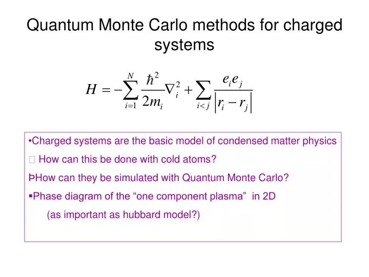
Quantum Monte Carlo methods for charged systems. Charged systems are the basic model of condensed matter physics How can this be done with cold atoms? How can they be simulated with Quantum Monte Carlo? Phase diagram of the “one component plasma” in 2D (as important as hubbard model?).

E N D
Quantum Monte Carlo methods for charged systems • Charged systems are the basic model of condensed matter physics • How can this be done with cold atoms? • How can they be simulated with Quantum Monte Carlo? • Phase diagram of the “one component plasma” in 2D • (as important as hubbard model?)
Which ensemble? T=0 VMC (variational) DMC/GFMC (projector) or T>0? PIMC (path integrals) Which basis? Particle Coordinate Space Sz representation for spin Occupation Number Lattice models Wave functions Hartree-Fock Slater-Jastrow Backflow, 3 body Localized orbitals in crystal Many different quantum Monte Carlo methods • Which Hamiltonian? • Continuum • Lattice (Hubbard, LGT)
Imaginary-time path integrals The thermal density matrix is: • Trotter’s theorem (1959):
“Distinguishable” particles within PIMC • Each particle is a ring polymer; an exact representation of a quantum wavepacket in imaginary time. • Integrate over all paths • The dots represent the “start” of the path. (but all points are equivalent) • The lower the real temperature, the longer the “string” and the more spread out the wavepacket. • Path Integral methods can calculate all equilibrium properties without uncontrolled approximations • We can do ~2000 charges with ~1000 time slices.
Bose/Fermi Statistics in PIMC • Average by sampling over all paths and over connections. • At the superfluid transition a “macroscopic” permutation appears. • This is reflection of bose condensation within PIMC. • Fermion sign problem: -1 for odd permutations.
Projector Monte Carlo (T=0)aka Green’s function MC, Diffusion MC • Automatic way to get better wavefunctions. • Project single state using the Hamiltonian • This is a diffusion + branching operator. • Very scalable: each walker gets a processor. • This a probabilityfor bosons/boltzmanons since ground state can be made real and non-negative. • Use a trial wavefunction to control fluctuations and guide the random walk; “importance sampling” • For a liquid we use a Jastrow wavefunction, for a solid we also use Wannier functions (Gaussians) to tie particles to lattice sites. • More accurate than PIMC but potentially more biased by the trial wavefunction.
How can we handle charged systems? • If we cutoff potential : • Effect of discontinuity never disappears: (1/r) (r2) gets bigger. • Will not give proper plasmons because Poisson equation is not satisfied • Image potential solves this: VI = v(ri-rj+nL) • But summation diverges. We need to resum. This gives the Ewald image potential. • For one component system we have to add a background to make it neutral (background comes from other physics) • Even the trial function is long ranged and needs to be resummed.
Computational effort O(N3/2) O(N) O(N3/2) O(N3/2) O(N1/2) O(1) • r-space part same as short-ranged potential • k-space part: • Compute exp(ik0xi) =(cos (ik0xi), sin (ik0xi)), k0=2/L. • Compute powers exp(i2k0xi) = exp(ik0xi )*exp(ik0xi) etc. Get all values of exp(ik . ri) with just multiplications. • Sum over particles to get k for all k. • Sum over k to get the potentials. Constant terms to be added. Table driven method used on lattices is O(N2). For N>1000 faster methods are known.
Fixed-node method • Impose the condition: • This is the fixed-node BC • Will give an upper bound to the exact energy, the best upper bound consistent with the FNBC. • f(R,t) has a discontinuous gradient at the nodal location. • Accurate method because Bose correlations are done exactly. • Scales well, like the VMC method, as N3. • Can be generalized from the continuum to lattice finite temperature, magnetic fields, …
Dependence of energy on wavefunction3d Electron fluid at a density rs=10Kwon, Ceperley, Martin, Phys. Rev. B58,6800, 1998 • Wavefunctions • Slater-Jastrow (SJ) • three-body (3) • backflow (BF) • fixed-node (FN) • Energy <f |H| f> converges to ground state • Variance <f [H-E]2f> to zero. • Using 3B-BF gains a factor of 4. • Using DMC gains a factor of 4. FN -SJ FN-BF
The 2D one component plasmaPRL 103, 055701 (2009); arXiv:0905.4515 (2009) • Electrons or ions on liquid helium • Semiconductor MOSFET • charged colloids on surfaces • We need cleaner experimental systems! • Bryan Clark, UIUC & Princeton • Michele Casula, UIUC & Saclay, France • DMC UIUC • Support from: NSF-DMR 0404853
Phase Diagram for 2d boson OCP(up to now) Hexatic phase G ~124 Classical plasma T (mR) Quantum-classical crossover Electrons on helium electrons Quantum fluid Wigner crystal 1 / rs =(density)1/2 rs ~ 60 ~ 3x1012 cm2 De Palo, Conti, Moroni, PRB 2004.
Inhomogenous phases Maxwell construction • Cannot have 2-phase coexistence at first order transition! the background forbids it • Jamei, Kivelson and Spivak [Phys. Rev. Lett. 94, 056805 (2005)] “proved” (with mean field techniques) that a 2d charged system cannot make a direct transition from crystal to liquid • a stripe phase between liquid and crystal has lower energy • Does not prove that stripes are the lowest energy state, only that the pure liquid or crystal is unstable at the transition assume Boltzmann statistics – no fermion sign problem. F area
snapshots 122<G<124 classical quantum Triangular lattice forms spontaneously in PIMC
Structure Factors PIMC Exper. Keim, Maret, von Grunberg. Classical MC
Hexatic order r He,Cui,Ma,Liu,Zou PRB 68,195104 (2003). Muto , Aoki PRB 59, 14911(1999) r
2d OCP Phase Diagram PRL 102,055701 (2009) Clausius-Clapeyron relation : First order transition is on “nose” Hexatic phase Classical plasma T (mR) Wigner crystal Quantum fluid 1 / rs
Transition order differs from KT? Internal energy vs T ? 2nd order 1st order T (mR) 1 / rs T(mR)
Unusual structure in peak of S(k) Could be caused by many small crystals rs=65, N=2248
Structures exist in transition region • Are structures real? Or an ergodic problem • Are they different from a liquid? • Can we make a ground state model? Not one that is energetically favorable.
2D Bose OCP superfluid Normal fluid hexatic • Wigner crystal T (mR)
2dOCP fermion Phase diagram • 2d Wigner crystal is a spin liquid. • Magnetic properties are nearly divergent at melting (2d) and (nearly) 2nd order melting. • But sign problem? UNKNOWN Quantum Fluid Super-conductor?
Polarization transition Phase Diagram of 3DEG • second order partially polarized transition at rs=52 like the Stoner model (replace interaction with a contact potential) • Antiferromagnetic Wigner Crystal at rs>105
Conclusions • Long-ranged interactions are not an intractable problem for simulation. • We have established the outlines of the OCP phase diagram for boltzmannons and bosons. • Evidence for intervening inhomogeneous phases is weak • Future work: fermi statistics – but the “sign problem” makes the fluid phases challenging (not hopeless). • The OCP is a good target for a “quantum emulator.” • With optical lattice+disorder one can reach some of the most important problems in CMP.