Download
1 / 12
120 likes | 362 Views
Sociology 601 Class 24: November 19, 2009 (partial). Review regression results for spurious & intervening effects care with sample sizes for comparing models Dummy variables F-tests comparing models Example from ASR. Review: Types of 3-variable Causal Models. Spurious

E N D
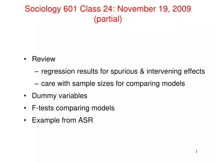
Sociology 601 Class 24: November 19, 2009(partial) • Review • regression results for spurious & intervening effects • care with sample sizes for comparing models • Dummy variables • F-tests comparing models • Example from ASR
Review: Types of 3-variable Causal Models • Spurious • x2 causes both x1 and y • e.g., age causes both marital status and earnings • Intervening • x1 causes x2 which causes y • e.g., marital status causes more hours worked which raises annual earnings • No statistical difference between these models. • Statistical interaction effects: The relationship between x1 and y depends on the value of another variable, x2 • e.g., the relationship between marital status and earnings is different for men and women.
Review: Regression models using Stata • see: • http://www.bsos.umd.edu/socy/vanneman/socy601/conrinc.do
Review: Regression models with Earnings Marital status, Age, and Hours worked.
Regression with Dummy Variables • Agresti and Finlay 12.3 • (skim 12.1-12.2 on analysis of variance) • Example: marital status, 5 categories • married • widowed • divorced • separated • never married
Regression with Dummy Variables: example • Example: marital status, 5 categories • married • widowed • divorced • separated • never married • . tab marital • marital | • status | Freq. Percent Cum. • --------------+----------------------------------- • married | 969 52.12 52.12 • widowed | 48 2.58 54.71 • divorced | 337 18.13 72.83 • separated | 98 5.27 78.11 • never married | 407 21.89 100.00 • --------------+----------------------------------- • Total | 1,859 100.00
Dummy Variables: stata programming * create 5 dummy variables from marital status: gen byte married=0 if marital<. replace married=1 if marital==1 gen byte widow=0 if marital<. replace widow=1 if marital==2 gen byte divorced=0 if marital<. replace divorced=1 if marital==3 gen byte separated=0 if marital<. replace separated=1 if marital==4 gen byte nevermar=0 if marital<. replace nevermar=1 if marital==5 * check marital dummies (maritalcheck should =1 for all nonmissing cases) egen byte maritalcheck=rowtotal(married widow divorced separated nevermar) tab marital maritalcheck, missing * shortcut method: tab marital, gen(mar) describe mar* * check new mar dummies (marcheck should =1 for all nonmissing cases) egen byte marcheck=rowtotal(mar1-mar5) tab marital marcheck, missin
Regression with Dummy Variables: example • . regress conrinc mar1-mar4 if sex==1 • Source | SS df MS Number of obs = 725 • -------------+------------------------------ F( 4, 720) = 9.78 • Model | 2.4002e+10 4 6.0006e+09 Prob > F = 0.0000 • Residual | 4.4177e+11 720 613572279 R-squared = 0.0515 • -------------+------------------------------ Adj R-squared = 0.0463 • Total | 4.6577e+11 724 643334846 Root MSE = 24770 • ------------------------------------------------------------------------------ • conrinc | Coef. Std. Err. t P>|t| [95% Conf. Interval] • -------------+---------------------------------------------------------------- • mar1 | 14111.68 2316.232 6.09 0.000 9564.302 18659.05 • mar2 | 11331.78 7143.717 1.59 0.113 -2693.223 25356.79 • mar3 | 6709.996 2970.39 2.26 0.024 878.3349 12541.66 • mar4 | 8404.298 5074.261 1.66 0.098 -1557.817 18366.41 • _cons | 31336.99 1958.271 16.00 0.000 27492.38 35181.59 • ------------------------------------------------------------------------------ • Omitted category = never married (mar5) • b1 = 14111; • Currently married men earn on average $14,111 more than never married men. • t= 6.09; p<001; so, statistically significant (more than single men).
Regression with Dummy Variables: example • . regress conrinc mar1-mar4 if sex==1 • Source | SS df MS Number of obs = 725 • -------------+------------------------------ F( 4, 720) = 9.78 • Model | 2.4002e+10 4 6.0006e+09 Prob > F = 0.0000 • Residual | 4.4177e+11 720 613572279 R-squared = 0.0515 • -------------+------------------------------ Adj R-squared = 0.0463 • Total | 4.6577e+11 724 643334846 Root MSE = 24770 • ------------------------------------------------------------------------------ • conrinc | Coef. Std. Err. t P>|t| [95% Conf. Interval] • -------------+---------------------------------------------------------------- • mar1 | 14111.68 2316.232 6.09 0.000 9564.302 18659.05 • mar2 | 11331.78 7143.717 1.59 0.113 -2693.223 25356.79 • mar3 | 6709.996 2970.39 2.26 0.024 878.3349 12541.66 • mar4 | 8404.298 5074.261 1.66 0.098 -1557.817 18366.41 • _cons | 31336.99 1958.271 16.00 0.000 27492.38 35181.59 • ------------------------------------------------------------------------------ • Omitted category = never married (mar5) • b2 = 11331; • Currently widowed men earn on average $11,331 more than never married men. • t= 1.59; p=.11; so, not statistically significant. • So, no earnings difference between widowed men and never married men.
Regression with Dummy Variables: example • . regress conrinc mar1-mar4 if sex==1 • Source | SS df MS Number of obs = 725 • -------------+------------------------------ F( 4, 720) = 9.78 • Model | 2.4002e+10 4 6.0006e+09 Prob > F = 0.0000 • Residual | 4.4177e+11 720 613572279 R-squared = 0.0515 • -------------+------------------------------ Adj R-squared = 0.0463 • Total | 4.6577e+11 724 643334846 Root MSE = 24770 • ------------------------------------------------------------------------------ • conrinc | Coef. Std. Err. t P>|t| [95% Conf. Interval] • -------------+---------------------------------------------------------------- • mar1 | 14111.68 2316.232 6.09 0.000 9564.302 18659.05 • mar2 | 11331.78 7143.717 1.59 0.113 -2693.223 25356.79 • mar3 | 6709.996 2970.39 2.26 0.024 878.3349 12541.66 • mar4 | 8404.298 5074.261 1.66 0.098 -1557.817 18366.41 • _cons | 31336.99 1958.271 16.00 0.000 27492.38 35181.59 • ------------------------------------------------------------------------------ • Omitted category = never married (mar5) • b3 = 6709.996; • Currently divorced men earn on average $6,710 more than never married men. • t= 2.26; p<.05; so, statistically significant (more than single men). • Note that b3 < b2, but b3 is statistically significant even though b2 is not. • High standard error of b2 (because few widowed men 25-54).
Inferences: F-tests Comparing models Comparing Regression Models, Agresti & Finlay, p 409: Where: Rc2 = R-square for complete model, R r2 = R-square for reduced model, k = number of explanatory variables in complete model, g = number of explanatory variables in reduced model, and N = number of cases.
Next: Regression with Interaction Effects • Examples with earnings: • age x gender • marital status x gender