Download
1 / 46
470 likes | 756 Views
Fast Set Intersection in Memory. Bolin Ding Arnd Christian König UIUC Microsoft Research. Outline. Introduction Intersection via fixed-width partitions Intersection via randomized partitions Experiments. Outline. Introduction Intersection via fixed-width partitions

E N D
Fast Set Intersection in Memory Bolin Ding Arnd Christian König UIUCMicrosoft Research
Outline Introduction Intersection via fixed-width partitions Intersection via randomized partitions Experiments
Outline Introduction Intersection via fixed-width partitions Intersection via randomized partitions Experiments
Introduction • Motivation: general operation in many contexts • Information retrieval (boolean keyword queries) • Evaluation of conjunctive predicates • Data mining • Web search • Preprocessing index in linear (to set size) space • Fast online processing algorithms • Focusing on in-memory index
Related Work |L1|=n, |L2|=m, |L1∩ L2|=r • Sorted lists merge • B-trees, skip lists, or treaps • Adaptive algorithms • Hash-table lookup • Word-level parallelism • Intersection size r is small • w: word size • Map L1 and L2 to a small range [Hwang and Lin 72], [Knuth 73], [Brown and Tarjan 79], [Pugh 90], [Blelloch and Reid-Miller 98], … (bound # comparisons w.r.t. opt) [Demaine, Lopez-Ortiz, and Munro 00], … [Bille, Pagh, Pagh 07]
Basic Idea Preprocessing: L1 Small groups 1. Partitioning into small groups Hash images 2. Hash mapping to a small range {1, …, w} Hash images w: word size Small groups L2
Basic Idea Two observations: L1 Small groups 1. At most r = |L1∩L2| (usually small) pairs of small groups intersect Hash images 2. If a pair of small groups does NOT intersect, then, w.h.p., their hash images do not intersect either (we can rule it out) Hash images Small groups L2
Basic Idea Online processing: L1 Small groups 1. For each possible pair, compute h(I1)∩h(I2) I1 Hash images 2.1. If empty, skip (if r = |L1∩L2| is small we can skip many); 2.2. otherwise, compute the intersection of two small groups I1∩I2 h(I1) Hash images h(I2) Small groups I2 L2
Basic Idea Two questions: L1 Small groups 1. How to partition? I1 Hash images 2. How to compute the intersection of two small groups? h(I1) Hash images h(I2) Small groups I2 L2
Our Results |L1|=n, |L2|=m, |L1∩ L2|=r , • Sets of comparable sizes • Sets of skewed sizes (reuse the index) • Generalized to k sets and set union • Improved performance (wall-clock time) in practice (compared to existing solutions) • (i) Hidden constant; (ii) random/scan access • Best in most cases; otherwise, close to the best (efficient in practice) (better when n<<m)
Outline Introduction Intersection via fixed-width partitions Intersection via randomized partitions Experiments
elements in each interval pairs of small groups Fixed-Width Partitions • Outline • Sort two sets L1 and L2 • Partition into equal-depth intervals (small groups) • Compute the intersection of two small groups using QuickIntersect(I1, I2) |L1|=n, |L2|=m, |L1∩ L2|=r w: word size
Subroutine QuickIntersect (Preprocessing) Map I1 and I2 to {1, 2, …, w} using a hash function h h Hash images are encoded as words of size w {1, 2, …, w} (Online processing) Computeh(I1)∩h(I2) (bitwise-AND) h (Online processing) Lookup 1’s in h(I1)∩h(I2) and “1-entries”in the hash tables Go back to I1 and I2 for each “1-entry” Bad case: two different elements in I1 and I2 are mapped to the same one in {1, 2, …, w}
Analysis (Preprocessing) Map I1 and I2 to {1, 2, …, w} using a hash function h h Hash images are encoded as words of size w {1, 2, …, w} (Online processing) Computeh(I1)∩h(I2) (bitwise-AND) h one operation |L1|=n, |L2|=m, |L1∩ L2|=r (Online processing) Lookup 1’s in h(I1)∩h(I2) and “1-entries”in the hash tables Go back to I1 and I2 for each “1-entry” Total complexity: |h(I1)∩h(I2)| = (|I1∩I2| + # bad cases) operations Bad case: two different elements in I1 and I2 are mapped to the same one in {1, 2, …, w} one bad case for each pair in expectation
Analysis |L1|=n, |L2|=m, |L1∩ L2|=r w: word size • Optimize the parameter a bit --- total # of small groups (|I1| = a, |I2| = b) s.t. --- ensure one bad case for each pair of I1 and I2 Total complexity:
Outline Introduction Intersection via fixed-width partitions Intersection via randomized partitions Experiments
Randomized Partition • Outline • Two sets L1 and L2 • Grouping hash function g (different from h): group elements in L1 and L2 according to g(.) • Compute the intersection of two small groups: I1i={x∈L1 | g(x)=i} and I2i={y∈L2 | g(y)=i} using QuickIntersect |L1|=n, |L2|=m, |L1∩ L2|=r w: word size The same grouping function for all sets g(x) = 1 g(x) = 2 … …
Randomized Partition • Outline • Two sets L1 and L2 • Grouping hash function g (different from h): group elements in L1 and L2 according to g(.) |L1|=n, |L2|=m, |L1∩ L2|=r w: word size The same grouping function for all sets g(x) = 1 g(x) = 2 … … g(y) = 1 g(y) = 2 … …
Analysis • Number of bad cases for each pair • Then follow the previous analysis: • Generalized to k sets Rigorous analysis is trickier
Data Structures • Multi-resolution structure for online processing • Linear (to the size of each set) space
A Practical Version • Outline • Motivation: linear scan is cheap in memory • Instead of using QuickIntersect to compute I1i∩I2i, just linear scan them, in time O(|I1i|+|I2i|) • (Preprocessing) Map I1i and I2iinto {1, …, w} using a hash function h • (Online processing) Linear scan I1i and I2ionly ifh(I1i)∩h(I2i) ≠ w: word size
A Practical Version • Outline • Motivation: linear scan is cheap in memory • Instead of using QuickIntersect to compute I1i∩I2i, just linear scan them, in time O(|I1i|+|I2i|) I1i h(I1i) Linear scan h(I2i) I2i
A Practical Version • Outline • Motivation: linear scan is cheap in memory • Instead of using QuickIntersect to compute I1i∩I2i, just linear scan them, in time O(|I1i|+|I2i|) I1i h(I1i) Linear scan h(I2i) I2i
Analysis • The probability of false positive is bounded: • Using p hash functions, false positive happens with lower probability: at most • Complexity • When I1i∩I2i = , (false positive) scan it with prob • When I1i∩I2i ≠ , must scan it (only r such pairs) Rigorous analysis is trickier
Intersection of Short-Long Lists • Outline (when |I1i|>>|I2i|) • Linear scan in I2i • Binary search in I1i • Based on the same data structure, we get L1: L2:
Outline Introduction Intersection via fixed-width partitions Intersection via randomized partitions Experiments
Experiments • Synthetic data • Uniformly generating elements in {1, 2, …, R} • Real data • 8 million Wikipedia documents (inverted index – sets) • The 10 thousand most frequent queries from Bing (online intersection queries) • Implemented in C, 4GB 64-bit 2.4GHz PC • Time (in milliseconds)
Experiments |L1|=n, |L2|=m, |L1∩ L2|=r • Sorted lists merge • B-trees, skip lists, or treaps • Adaptive algorithms • Hash-table lookup • Word-level parallelism • Intersection size r is small • w: word size • Map L1 and L2 to a small range [Hwang and Lin 72], [Knuth 73], [Brown and Tarjan 79], [Pugh 90], [Blelloch and Reid-Miller 98], … (bound # comparisons w.r.t. opt) [Demaine, Lopez-Ortiz, and Munro 00], … [Bille, Pagh, Pagh 07]
Experiments Merge • Sorted lists merge • B-trees, skip lists, or treaps • Adaptive algorithms • Hash-table lookup • Word-level parallelism SkipList Adaptive SvS Hash Lookup BPP
Experiments • Our approaches • Fixed-width partition • Randomized partition • The practical version • Short-long list intersection
Experiments • Our approaches • Fixed-width partition • Randomized partition • The practical version • Short-long list intersection IntGroup RanGroup RanGroupScan HashBin
Varying the Size of Sets |L1|=n, |L2|=m, |L1∩ L2|=r n = m = 1M~10M r = n*1%
Varying the Size of Intersection |L1|=n, |L2|=m, |L1∩ L2|=r n = m = 10M r = n*(0.005%~100%) = 500~10M
Varying the Ratio of Set Sizes |L1|=n, |L2|=m, |L1∩ L2|=r m = 10M, m/n = 2~500 r = n*1%
Conclusion and Future Work • Simple and fast set intersection algorithms • Novel performance guarantee in theory • Better wall-clock performance:best in most cases; otherwise, close to the best • Future work • Storage compression in our approaches • Select the best algorithm/parameter by estimating the size of intersection (RanGroupv.s. HashBin)(RanGroupv.s. Merge) (parameter p) (sizes of groups)
Compression (preliminary results) • Storage compression in RanGroup • Grouping hash function g: random permutation/prefix of permuted ID • Storage of short lists suffix of permuted ID • Compared with Merge algo on d-compression of inverted index • Compressed Merge: 70% compression, 7 times slower (800ms) • Compressed RanGroup: 40% compression, 1.5 times slower (140ms)
Remarks (cut or not?) • Linear additional space for preprocessing and indexing • Generalized to k lists • Generalized to disk I/O model • Difference between Pagh’s and ours • Pagh: Mapping + Word-level parallelism • Ours: Grouping + Mapping
Data Structures (remove) Linear scan
Number of Lists (skip) size = 10M
Number of Hash Functions (remove) p = 1 p = 2 p = 4 p = 6 p = 8
Compression (remove) n = m = 1M~10M r = n*1%
Intersection of Short-Long Lists • Outline • Two sorted lists L1 and L2 • Hash function g: Group elements in L1 and L2 according to g(.) • For each element in I2i={y∈L2 | g(y)=i}, binary search it in I1i={x∈L1 | g(x)=i} (Preprocessing) (Online processing) L1: L2:
Analysis • Online processing time • Random variable Si: size of I2i • E(Si) = 1; • ∑i |I1i| = n; • concavity of log(.) • Comments: • 1. The same performance guarantee as B-trees, skip-lists, and treaps • 2. Simple and efficient in practice • 3. Can be generalized for k lists
Data Structures Random access Linear scan