Download

1 / 54
540 likes | 733 Views
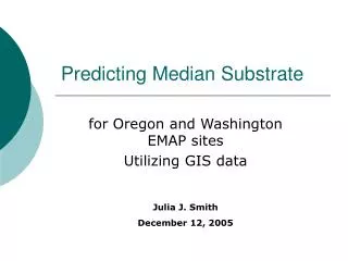
Predicting Median Substrate. for Oregon and Washington EMAP sites Utilizing GIS data. Julia J. Smith December 12, 2005. Why Predict Median Substrate?. Indicator of overall stream health Bed load transport Stream Power Microinvertebrate habitat Fish habitat

E N D
Predicting Median Substrate for Oregon and Washington EMAP sites Utilizing GIS data Julia J. Smith December 12, 2005
Why Predict Median Substrate? Indicator of overall stream health • Bed load transport • Stream Power • Microinvertebrate habitat • Fish habitat • How is human development affecting a stream
What is LD50? LD50 is a measure of median substrate. • Geometric mean of class boundaries • Log10 of the geometric means • Several samples at each site • LD50 is the median value of log10(geometric mean of class)
Geomorphic Metrics is the total bank-full shear stress s is the density of sediment is fluid density g is gravitational acceleration h is bank-full depth S is channel slope
Geomorphic Metrics Distance-weighted Stream Power versus LD50 r = 0.327, p-value = 2.63 x 10 -12
Geomorphic Metrics Outlet link mean slope versus LD50 r = 0.214, p-value = 3.78 x 10⁻⁶
Geologic Metrics Percent Unconsolidated Geologic type versus LD50 r = -0.246, p-value = 1.18 x 10⁻⁷
Climatic Metrics Annual average precipitation versus LD50 r = 0.199, p-value = 1.56 x 10⁻⁶
Climatic Metrics Average annual potential evapotranspiration (mm) versus LD50 r = -0.046, p-value = 0.342
Land Cover Metrics 1. Developed 2. Barren 3. Forest 4. Grasses 5. Agriculture 6. Wetlands 7. Open water/perennial ice and snow 8. Shrubland
Land Cover Metrics Percentage of watershed that is forest versus LD50 r = 0.19, p-value = 3.516 x 10⁻⁵
Distance-Weighted metrics • j represents the land cover type of concern, • Ajrepresents the total area for land cover type j in the watershed, • represents the coefficient of exponential decay, represents average distance from outlet for land cover of type j n represents the total number of the land cover types
Additional Land Cover Metrics • Buffered Metrics – Buffered within a measure of the stream (30 meters, 100 meters, 300 meters) • Buffered and Distance-weighted metrics
Goals • Predict LD50 without visiting sites • Small number of predictors for scientifically sensible model
Methods-Stepwise Variable Selection • Multiple Linear Regression • Top-in-tier models • Top geomorphic models plus one from each of the remaining tiers
Akaike’s Information Criterion N observations p predictors RSS is the sum of squared residuals
AIC in stepwise variable selection Forward Stepwise Selection - Method for choosing the top predictor from each tier Start with the intercept model Choose the variable that reduces AIC the most and include in model. Stepwise selection in both directions- Method chosen for choosing all top Geomorphic predictors Start with full model. Add and subtract variables until the model with minimum AIC is found or iteration stops.
Methods: CART Classification and Regression Trees Predicted Response:
Hybrid of Multiple Linear Regression and CART • Utilize CART on the residuals • Add indicator variables to the multiple linear regression equation for one minus the number of terminal nodes in the tree • Create new multiple regression model with variables and indicator variables
Analysis Comparison – Top 4-tier Models • Problems with top 4-tier models • Low Adjusted R2 • Low Predictive Ability • Over-prediction and under-prediction of fine and bedrock substrate • Non-normal residuals • Benefit of top 4-tier models • Small number of predictors
Analysis Comparison – Geomorphic plus Top 3-Tier Models • Problems with top geomorphic plus top 3-tier model • Increase in number of variables • Predictive ability still low • Over-prediction and under-prediction of fine and bedrock substrate • Some collinearity between variables
Analysis Comparison – Geomorphic plus Top 3-Tier Models • Benefits with top geomorphic plus top 3-tier model • Improved predictions • Improved normality of residuals
Comparison of Analysis - CART • Problems with CART • Low predictive-ability • Predicts several observed substrate sizes in one node • Over-prediction and under-prediction of fines and bedrock substrate • Omitting one site creates different tree • Benefits of CART • Simple analysis • Missing variables not an issue
Comparison of Analysis-Hybrids • Problems with hybrid models • Increased number of variables • Collinearity with introduction of node indicator variables • Non-normal residuals
Comparison of Analysis-Hybrids • Benefit of hybrid models • Residuals closer to normal • Increased predictive-ability • Explains some of the variation created by fitting a linear model to ordinal data
One example: Residual Tree forHybrid Geomorphic plus Top 3-Tier Model Most promising multiple regression prediction model: Geomorphic plus top 3-tier
One example: Residual Tree forHybrid Geomorphic plus Top 3-Tier Model
One example: Observed vs. Predicted forHybrid Geomorphic plus Top 3-Tier Model Plot of predictions against observed LD50
Coast Range Ecoregion • Less skewed distribution of LD50 • No measurements are outliers • Similar ecosystem throughout region
Top 4-Tier Coast Range Model • Predictors • Average aspect (climatic) • Average watershed elevation (geomorphic) • % watershed as volcanic geologic type (geologic) • % wetlands (distance weighted and buffered)
Coast Range ModelTop Geomorphic Variables • Average watershed elevation (m) • Drainage density • Mean slope within a 300-meter buffer • Ratio of width of stream to width of floodplain • Coefficient of average hill connectivity • Distance to the first tributary (m) • Percent of landscape with less than 4% slope • Percent of landscape with less than 7% slope • Measure of size and complexity of river • Percent of stream as cascade • Distance-weighted stream power • Watershed relief divided by its length
Observed versus Predicted: Coast Range Geomorphic + Top 3-Tier
CART - Coast Range Ecoregion Predictions versus Observed LD50
Coast Range: Hybrid Models • Benefits of hybrid • Improved prediction • Improved fit • Improved normality of residuals • Problems with hybrid • Increased number of predictors • Collinearity with node indicator variables