Download
1 / 47
470 likes | 707 Views
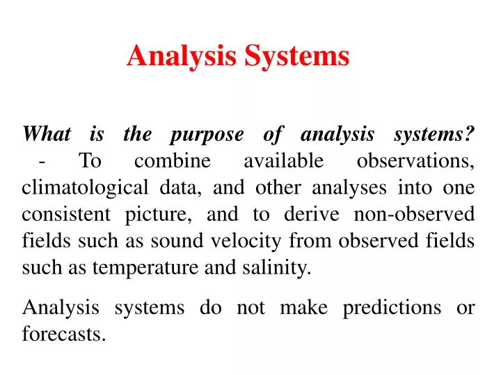
Analysis Systems. What is the purpose of analysis systems? - To combine available observations, climatological data, and other analyses into one consistent picture, and to derive non-observed fields such as sound velocity from observed fields such as temperature and salinity.

E N D
Analysis Systems What is the purpose of analysis systems?- To combine available observations, climatological data, and other analyses into one consistent picture, and to derive non-observed fields such as sound velocity from observed fields such as temperature and salinity. Analysis systems do not make predictions or forecasts.
Analysis Systems • What are the Navy’s Ocean Analysis Systems? • MODAS – Modular Ocean Data Assimilation System • OTIS – Optimum Thermal Interpolation System • MVOI – Multivariate Optimum Interpolation
MODASModular Ocean Data Assimilation System Primary contacts: Dan Fox (NRLSSC), Martin Booda (NAVO) MODAS was developed at the Naval Research Lab at Stennis Space Center in the 1990’s (Fox et al., 2002). It is currently used in a stand-alone mode and also to initialize a relocatable version of the Princeton Ocean Model. A subset of the full capabilities is available for use on submarines.
MODAShttp://www7320.nrlssc.navy.mil/modas/ Analysis system that uses optimal interpolation to incorporate MC-SSTs, SSH from satellite altimetry, T and S data from profilers (XBTs and CTDs) and fixed or drifting buoys, with climatological data to produce 3D T and S fields. 3D sound velocity fields, and associated acoustic parameters, and geostrophic velocity fields, are derived from the temperature and salinity fields.
Physics • Geostrophic. In water depths greater than the reference level, geostrophic velocities are referenced to the reference level. In water depths less than the reference level, geostrophic velocities are referenced to the bottom, i.e. it is assumed that there is no horizontal pressure gradient at the bottom, which can produce a velocity field that is locally divergent. Strictly speaking, the geostrophic velocity field should be non-divergent. The reference level is user-selectable. The default is 1000 m.
Domain • Determined by user The EOF scheme used to compress the 3D temperature and salinity output has a limit of 360 grid points in the east-west direction and 181 grid points in the north-south direction. The spatial resolution, in combination with the maximum number of grid points, sets the maximum allowable domain, if the EOF-compressed output is needed.
Spatial Resolution • Determined by user as a result of specifying the domain size, and the number of grid points or the spatial resolution: xmin: longitude at the left edge of the grid (+E, -W) xmax: longitude at the right edge of the grid ymin: latitude at the bottom edge of the grid (+N, -S) ymax: latitude at the top edge of the grid nx: number of grid points in the east-west direction (max = 360) ny: number of grid points in the north-south direction (max = 181)
E-W grid spacing: dx = (xmax - xmin) / (nx - 1) N-S grid spacing: dy = (ymax - ymin) / (ny - 1) # grid ptsE-W dir. nx = 1 + (xmax-xmin)/dx # grid ptsN-S dir. ny = 1 + (ymax-ymin)/dy If specifying, dx and dy, program will calculate nx and ny, and GUI will alert user if nx, ny aren’t integers. From the MODAS 2.1 User's Manual, applies to the GUI-based version. Try out the Interactive MODAS Grid Calculator
Temporal resolution • None This is not a time-stepping predictive model. The analysis can be updated at whatever interval the user chooses, but should be based on the availability of new data to assimilate. NAVO’s update cycle is generally once per day.
Initialization • The user has the option of using a previous MODAS run as the first guess or using climatology. MODAS2.1 has its own climatology. The MODAS climatology is based on a blend of MOODS T and S data in the upper 1500 m of the ocean with the Levitus climatology in the deeper ocean. The MODAS climatology is stored as bimonthly T and S at 37 depth levels from 0 to 6500 m, on a grid with horizontal resolution ranging from 1/2 in the open ocean to 1/4 in coastal seas and 1/8 near the coasts. The MODAS climatology extends into water depths as shallow as 5 m.
Data Assimilation • Assimilates SSH, SST, XBTs, fixed buoys, and PALACE floats at this time (May 2002). • There is a time window over which data is assimilated – in other words how far back in time should data be included and with what weighting. This time window is not easily changed, or viewable, by the user, but can be accessed and modified. • 1/8° resolution global field of SSH is supplied by the altimetry data fusion center (ADFC). Does not improve solution in all regions (due to seiching, among other things), so is not used everywhere.
Altimetry Processing Upgrade: “CLAM II” * Implements “moving covariance” function in MODAS OI (more continuity of features between tracks) Original Results Updated Results Courtesy of John Harding, NRL-SSC Note particularly significant improvement in these areas Note sampling impact: Red would be green but for this area
Clam Shallow Water Evaluation Most Accurate Modas First-Guess Field (Bottom Depth < 200 m) MODAS Seasonal Climatology MODAS Climatology - MCSST’s Latitude Longitude
Adriatic Arabian Sea Gulf of Alaska/Eastern Aleutians Gulf of Cadiz Central Med Central North Atlantic Eastern Med Greenland/Iceland/ Norwegian Sea Kamchatka Mediterranean regional Bay of Biscay/NE Atlantic Northeast Pacific Gulf of Oman/Arabian Gulf SOCAL Straits of Sicily Western Med NAVO MODAS areas not using SSH(as of 7/3/02)
Data Assimilation (con’t.) • 8.8 km resolution MC-SST, derived from 2x2 blocks of 4.4 km Global Area Coverage (GAC) data • Relationships between SSH and subsurface T, and SST and subsurface T, based on historical data, are used together with climatology to produce synthetic vertical profiles of T, down to a depth of 1500 m. • After SSH and SST have been used to create the “dynamic climatology”, in-situ data from XBTs, CTDs, buoys and floats is assimilated through an optimal interpolation (OI) scheme. The 3D grid of T is then modified near the surface by using an analysis of mixed layer depths. T/S relationships are then used to produce a 3D S field as well. If S observations are available, they are then used to modify the first guess salinity field.
MODULAR OCEAN DATA ASSIMILATIONSYSTEM MOODS Profiles MODAS Climatology Satellite Measured SSH and SST Green line represents profile derived only using satellite measured height and temperature Decades of edited MOODS profiles are used to derive statistical relationships between surface height and temperature and subsurface temperature and salinity Relationships are stored on an irregular mesh, varying from 1 to 1/8 degree in resolution to permit high resolution analyses in shallow water regions Climatology MODAS Synthetic Final Analysis In Situ BT Courtesy of Dan Fox, NRL-SSC
AXBT Temp SSH + SST + Clim Climatological Temp MODAS Validation Example: AXBT Survey MODAS results Cold core eddy MODAS Temperature at 200m Courtesy of Dan Fox, NRL-SSC
T/S plot from central California1997-2002 Equatorial Intermediate Water Temperature (C) El Nino affect North Pacific Intermediate Water 31 33 31 34 35 Salinity
Implementation • Set of Fortran programs and UNIX scripts run under the UNIX operating system. Different versions of MODAS have different subsets of the full suite of modules installed. • MODAS modules have been "wired together" to produce several analysis and forecast systems presently running at various Navy facilities. Versions designed for shipboard and submarine-based users are under development now. • PC-IMAT now includes MODAS-Lite, basically the same version as is run at the METOC centers, but with different GUI and Perl scripts.
MODULAR OCEAN DATA ASSIMILATIONSYSTEM Versions: Central Site, METOC Center, On Scene MODAS2.1 “Heavy” Run at NAVOCEANO on SGI Origin, Power Challenge Array, and ONYX systems Satellite altimetry and MCSSTs plus in situ data Includes reloctable Princeton Ocean Model Approx 6 GB of disk space required MODAS2.1 : NITES-I ASHORE METOC Center version All capabilities of above except would normally receive first guess field from NAVO via TEDS METCAST. Variable disk space (max 6 GB) depending on desired area of coverage UNIX systems (HP TAC4, Sun, SGI, PC LINUX, …) MODAS2.1 : NITES-I AFLOAT (“MODAS/Lite”) No direct altimetry use. Requires first guess field from MODAS run at Center. Input/output via TEDS database Minimal disk space required ( less than 1 GB for global coverage ) UNIX systems (as above)
MODAS 2.1 OUTPUT PRODUCTS ZNR UUUUU O 281742Z OCT 98 MSGID/NAVO/GRIDFLD/1504/OCT PROD/OCEANMET/281742Z4/OCT/000/1OF1 GRID/3100N4/04700E1/0M/133/97/34/0.068DEG/0.083DEG/VAR/03 NARR/UNCL prgars MODAS2 TEMPERATURE 98301 981028 8 5 133 1 97 97 - 2.027655125 1.865198374 :I8:U98:D9.875420ZYXVUTSSRR.Q.POMMKJIHG.E.DCC.B:JA:DB:DC.DEE LMMRW027CHJQW2556795ZUTMEBLYGQ5CTXJL0JLX1JO7WQ0CVE82O9ZCQZG7WPXY5OD0 20.210847855 :KB:YA.B.CDDEGGHHIIJJKLMMOOPQRSTTUUVVWXX.YZ01223344.5:D677668:M9:E8: JJXX 28108 0000/ 12930 04800 88888 00275 MODAS JJXX 28108 0000/ 13000 04800 88888 00276 MODAS JJXX 28108 0000/ 12830 04830 88888 00292 03291 08290 MODAS JJXX 28108 0000/ 12900 04830 88888 00283 03282 08281 13280 MODAS JJXX 28108 0000/ 12930 04830 88888 00279 03279 08279 MODAS JJXX 28108 0000/ 12800 04900 88888 00294 03293 MODAS JJXX 28108 0000/ 12830 04900 88888 00293 03292 08292 13290 18286 MODAS JJXX 28108 0000/ 12900 04900 88888 00291 03291 08290 13289 18288 MODAS JJXX 28108 0000/ 12930 04900 88888 00286 03285 08285 13286 18285 MODAS Text/Binary/Message Files: • Byte-Encoded & EOF-Compacted Temperature/SV (also pushed to centers, facilities & ships at sea) • JJXX/JJYY/KKXX Synthetic BTs • OVLY2 of Physical/Acoustic parameters • NetCDF of Temperature/SV/Salinity • ARCVIEW Format (for REACTs) Physical/Acoustic Graphics: • Temperature Contours at Depth • Currents over Temperature at Depth • DSCA, SSCA, MLD, SLD, ZX • Observations Chart (Secret) Wavelet-compressed fields became available in May 2001
Note that velocity scale is different for every picture MODAS
The arrows are parallel to the streamlines everywhere and their length indicates the speed, as referenced to the velocity scale vector. The length of the curved arrow is a function of the velocity all along it's short path - not just at the beginning.
Typical Satellite SSTs of Kuroshio Current (2/19/1996) Estimated surface current conditions in Kuroshio area during time period of the MODAS data analysis. Data are from weekly survey reports produced by Japanese researchers. These reports are independent of MODAS calculations, though the same data may be used. Adapted from Johnson and Broome 1999
References Fox, D. N., W. J. Teague, C. N. Barron, M. R. Carnes, and C. M. Lee, 2002: The Modular Ocean Data Assimilation System (MODAS). Journal of Atmospheric and Oceanic Technology, 19, 240-252. Fox, D.N., C.N. Barron, M.R. Carnes, M. Booda, G. Peggion, and J. Gurley, The Modular Ocean Data Assimilation System, Oceanography, 15 (1), 22-28, 2002a. Johnson, A. and R. Broome, 1999: Validation Test Report for the Modular Ocean Data Assimilation System (MODAS 2.1), 42 pp. Naval Research Laboratory, P. S. I., 1999: User's Manual for the Modular Ocean Data Assimilation System (MODAS) Version 2.1. PSI Technical Report S-285.
OTISOptimum Thermal Interpolation System Primary contact: Webb DeWitt (FNMOC) OTIS predates MODAS. It was developed at FNMOC in the 1980’s. While it is still being run by FNMOC, it is scheduled to be phased out.
OTIShttp://www.fnmoc.navy.mil/ • OTIS is an optimum interpolation (OI) based objective analysis scheme designed to produce analysis or "nowcasts" of temperatures in the upper 5000 m of the ocean. • OTIS does not provide currents as output, but feeds into TOPS (see below), which does.
Domain OTIS has been implemented at FNMOC on a variety of regional (eddy resolving) and global (non-eddy resolving) grids.
Temporal and Spatial Resolution • This is not a time-stepping predictive model. • Presently, SST-only runs are done for the global domain twice a day at 1 by 1 horizontal resolution, and once a day at 0.25 by 0.25. There is also a global 3D OTIS with 1 resolution run twice a day. Regional 3D runs are done once per day for the Atlantic and Pacific oceans using 0.2 by 0.2 resolution. • 34 levels are used in the vertical, with 5 m spacing near the surface, expanding to 100 m at 400 m depth and 200 m at 2000 m depth.
Initialization • The 3D implementation uses GDEM climatology as a starting point and then uses a real-time "ocean bogus" database. This is a significant difference from the way MODAS works. The "ocean bogus" is the fronts and eddies, or Oceanographic Features Analysis product, from NAVO. It gives positions of ocean features determined from satellite data, and each grid point in OTIS is assigned a water mass classification based on its position relative to these features. "The water mass classification determines the appropriate water mass climatology model to apply at the grid point" (Cummings et al. 1997). The water mass climatology model uses date, location, and remote and in-situ measurements, to determine the temperature and salinity versus depth for that grid point. • The OTIS SST-only runs use the previous analysis as the first guess field.
Data Assimilation • OTIS makes full use of the global real-time observations received at FNMOC. This includes, ships, fixed and drifting buoys, and satellite-derived sea surface temperatures, and bathythermograph and buoy subsurface temperatures. All observations are quality- controlled prior to being assimilated by OTIS. • The 2D and 3D versions may use different time windows over which they accept observations.
Output • Global OTIS SST may be viewed on the FNMOC web site (www.fnmoc.navy.mil). • Other OTIS fields are available as JMV thumbnails, or could be requested via Metcast, and viewed with JMV.
References Cummings, J. A., C. Szczechowski, and M. Carnes, 1997: Global and regional ocean thermal analysis systems. Marine Technology Society Journal, 31, 63-75. Documents on FNMOC web site.
3D-MVOI3-Dimensional Multivariate Optimum Interpolation Primary contact: Jim Cummings (FNMOC) 3D-MVOI was developed at NRL Monterey in the late 1990’s.
3D-MVOI • Currently being used in a 2D mode to provide SST to the operational COAMPSTM, the Coupled Ocean-Atmosphere Model Prediction System, and its regional versions DAMPS (Distributed Atmospheric Model Prediction System) or TAMS/RT. • Ultimately, 3D-MVOI will serve as the ocean data assimilation scheme feeding the predictive ocean models (NCOM regionally and POP globally) that will be coupled to the atmospheric models (COAMPSTM regionally and NOGAPS globally).
Domain Must match domain of atmospheric or ocean model that it’s being used with.
Ocean Forecast Component Sequential Incremental Update Cycle Analysis-Forecast-Analysis Ocean Obs MCSST GOES SST Ship SST Buoy SST XBT, CTD PALACE Float Fixed Buoy Drift Buoy Altim SSHA SSM/I Sea Ice Ocean QC Innovations 3D MVOI Increments Ocean Model First Guess Forecast Fields Prediction Errors MVOI - simultaneous analysis 5 ocean variables temperature, salinity, geopotential, velocity (u,v) Courtesy of Jim Cummings, NRL-Monterey
Initialization • A nowcast of the observed state is obtained by combining new observations with a background field. The background field can be from a short-term model forecast or a previous analysis (warm start), or climatology (cold start). The use of a previous analysis as the background field implies a persistence forecast from the last time the analysis was executed.
Operational Observation Data SourcesNRL Coupled Systems • Satellite SST~330,000 obs/day • satellite SST retrievals (NOAA 16) • In Situ SST/SSS~15,000 obs/day • surface ship, fixed and drifting buoys, CMAN, TRACKOB • Subsurface Temperature and Salinity Profiles~500 obs/day • XBTs, CTDs (TESACS), PALACE floats • fixed buoys (TAO, PIRATA), thermistor chain drifting buoys • Sea Surface Height Anomaly (SSHA)~100,000 obs/day • altimeter (TOPEX, ERS2, GFO), in situ observations (PALACE floats) • Sea Ice Concentration~1,2000,000 obs/day • SSM/I (DMSP F13, F14, F15) • Synthetic Salinity-Temperature-Depth Profiles (STDs) • temperature profiles computed from SST and SSHA, salinity computed from temperature (using MODAS databases) • synthetic profiles are generated in a sampling pattern to capture analyzed changes in SSHA that exceed ~2 cm Note that the type and amount of data is subject to change depending on what is available. (Slide is courtesy of Jim Cummings, NRL-Monterey)
Data Assimilation • In addition to numerous satellite and in-situ observations, MVOI uses synthetic temperature and salinity profiles calculated using the same databases and algorithms as MODAS, to project satellite sea surface height and temperature data down to the subsurface ocean. • A sophisticated interpolation scheme, which varies the weighting of the observations as a function of variable type, time, depth and horizontal distance is used.
Horizontal Correlation Length Scales NRL Coupled Systems Rossby radius of deformation (from Chelton et al. (1998), JPO 28: 433-460). Used as default for horizontal correlation length scales in the 3D-MVOI. Scales range from ~10 km at the poles to ~240 km in the tropics. Courtesy of Jim Cummings, NRL-Monterey
Data Assimilation (cont.) • Another method that is used to incorporate the SSH into the analysis is to adjust the model T and S fields to improve the agreement between the observed and modeled SSH field. This has the advantage of not always trying to restore the modeled field towards climatology.
References Cummings, J., 2002. Powerpoint brief.