Download
1 / 32
320 likes | 435 Views
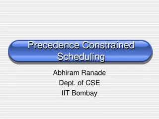
Precedence Constrained Scheduling. Abhiram Ranade Dept. of CSE IIT Bombay. Input. Directed Acyclic Graph G, #processors p. A. G. E. , 3. B. F. H. C. Vertex = unit time task edge (u,v) : Time(u) < Time(v). D. Output: Schedule. Time 1 2 3 4

E N D
Precedence Constrained Scheduling Abhiram Ranade Dept. of CSE IIT Bombay
Input • Directed Acyclic Graph G, #processors p A G E , 3 B F H C Vertex = unit time task edge (u,v) : Time(u) < Time(v) D
Output: Schedule Time 1 2 3 4 Processor 1 A D E G Processor 2 B F H Processor 3 C Schedule Length, to be minimized
Applications Project management. Vertex = lay foundation, build walls. Edges: what happens first to what happens later. Processors : Number of workmen. MS Project, others. Our problem: Simplified version. Other applications: Parallel computing.
Summary of results • Polytime algorithm when p=2. [Fuiji.. 69] • NP-hard for variable p. [LenKan 78] • NP-hardness not known for fixed p > 2. • Polytime algorithm for trees. [Hu 61]
Summary of results - 2 • Any greedy algorithm gives 2 - 1/p approximation. i.e. Schedule of length at most (2 - 1/p) times Optimal length. • [Coffman-Graham 72, Lam-Sethi 77] give 2 - 2/p approximation algorithm. • [Gangal-Ranade 08] give 2 – 7/(3p+1) approximation for p > 3.
Outline • Elementary Lower Bound ideas • Elementary algorithm and analysis • Deadline Constraints [GarJoh 76] • More complex problem, but generates new ideas. • 2 processor optimality, also without deadlines • Essentially gives 2 - 2/p approximation • Ideas behind 2 - 7/(3p+1) approximation algorithm
Elementary Lower Bounds • To prove optimality of any algorithm, need to show why it cannot be improved, i.e. lower bound on schedule length. • OPT H = Length of longest path in G. • OPT [ N / p ], N = #nodes [ x ] = ceiling(x), smallest integer x. Example: H = 3, [N/p] =[8/3] = 3
Generic Algorithm • Assign suitable “priority” to each vertex. • Of all “ready” vertices pick one with least priority value, and schedule it at earliest possible time slot. • Repeat until done. ready = no predecessors yet unscheduled. earliest possible = after predecessors.
Priority Example • Priority(v) = length of longest path from v. • Intuition: If many nodes depend upon me, then I should go first.
Proof of 2 approximation • Full (time-) slot: All processors busy • Number of “full” slots N/p • Number of partial slots H. Why? • Partial slot: Some processor did not get work. • All maximally long paths must shrink. • This can happen only H times. • Time N/P + H OPT + OPT = 2 OPT • Improve to 2 - 1/p. Priority?
Deadline Constraints [GarJoh 76] • Additional Input: Deadline D(v) : time by which v must be processed. • Need a schedule with p processors in which precedence constraints and deadlines are respected.
Deadline Propagation • v has N(d) descendants with deadline d v must itself finish by d - [N(d)/p]. new deadline: d(v) = min( D(v), mind d -[N(d)/p] ) • In what order to calculate? • (u,v) edge d(u) < d(v) • GJ Algo: priority = deadline. Optimal for p=2!
Example 4 4 d(A) = 4 - [7/5] = 2 d(B) = min(4-[8/5], 2-[1/5]) = 1 d(C) = …. = 3 d(D) = = 2 d(E) = . . . = 0 . B A . E D C . . 4
GJ Deadline Properties • Deadline < 1 : schedule not possible. • Optimal Schedule length Max deadline - Min deadline + 1. Example: 4 - 0 + 1 = 5 • Load bound : [N/p] = [17/5] = 4 • Longest path: H = 4 • Is this the best lower bound?
GJ Longest Path Bound (u,v) is edge d(u) < d(v) Path u to v of length H d(u) < d(v) - H H < Max Deadline – Min Deadline
GJ Load Bound Add a universal parent z d(z) Max deadline – [Number of descendants with Max deadline/p] = Max – [N/p] Min deadline Max – [N/p]
Scheduling without external deadlines • Set d(terminal vertices) = k, some number. • Propagate deadlines. m = least deadline. • Schedule from time m using deadlines. Theorem: Algorithm is optimal for p=2.
2 Processor Optimality • v : earliest scheduled vertex not meeting deadline • w : latest scheduled vertex before v scheduled alone. Always exists? Nodes in region must be Descendants of w. Time: 1 2 3 t’ t Proc 1: w v Proc 2: - Region has 2(t-t’)-1nodes with Deadline t-1. • d(w) t’, d(v) t-1 d(w) t-1 - (2(t-t’)-1)/2 = t’-1 Contradiction
Remarks • Why does this not work for p > 2? • Algorithm gives 2 - 2/p approximation for even p. More complex proof.
Improvements to GJ [GR 09] • Node v has N(d,L) descendants at distance at least L+1 having deadline at least d • Then d(v) mind,L d - L - [N(d,L)/p]
Example 4 d(A) = 4 - [7/5] = 2 d(B) = min(4-[8/5], 2-[1/5]) = 1 d(C) = …. = 3 d(D) = = 2 d(E) = . . . = 0 d(E) 4 – 2 – [12/5] = -1 Max - min + 1 = 6.Optimal! 4 . B A . E D C . . 4
Algorithm [GR 08] • Set d(terminal vertices) = 0 • Propagate deadlines. New rule. • For each v in non-decreasing deadline order: • (Rearrange ancestors of v if possible). • Schedule v in earliest possible slot, and smallest numbered processor.
Rearrange ancestors of v • Suppose t = last slot with ancestors of v. • Suppose vertices in slots t-1,t have same deadline. • Suppose v has < p ancestors in t-1,t. • Then move ancestors of v to slot t-1, move other vertices to slot t. • If slot t is not full, v can be scheduled in t.
Analysis Outline • Key part of proof: If algorithm constructs a long schedule, then deadline must drop a lot moving from last column to first. • Max deadline - min deadline + 1 optimal schedule length. • Optimal schedule must also be long, so good approximation factor.
How deadline varies in the schedule Time> 1 2 3 …. u v w 1 2 3 . . p Deadline can only increase in first row: d(u) d(v) Deadline can only increase in any column: d(u) d(w)
Partial slot rule 1 1 2 3 ….increasing time. u v w x y - - 1 2 3 . . p Deadline must increase in first row after a partial slot: d(u) < d(v) … why was not v scheduled earlier?
Partial slot rule 2 1 2 3 ….increasing time. u1 v u2 … uk - - 1 2 3 . . p Let M denote the number of nodes scheduled after u1..uk. Then d(u1) d(v) - [[M/k]/p]
Analysis Details • Count number of 1-slots, 2-slots, full slots present in schedule. • Relate counts to deadline drop, using rules discussed. • Find patterns of slot occupancies. • Special rules for specific patterns. • Combine estimates and take best.
Intuition: Easy schedules • Suppose all slots are partial: drop per slot. • Thus total deadline drop = length of schedule. • Optimal! • Suppose all slots are either 1 slots or full slots. • Partial slot rule 2 gives optimality.
Intuition: Difficult Schedules • Schedules with mixture of 2-slots and full slots. • Extreme case 1: 2-slots at the beginning, full slots at the end. • Extreme case 2: 2 slots and full slots alternate. • Omitted. See paper.
Concluding Remarks • Analysis is complicated, but not much more than 2-2/p analysis of Lam-Sethi. • Algorithm is simpler than Coffman-Graham. • Technique will not work beyond 2 - 3/p. Even getting there is hard.


![W[2]-hardness of precedence constrained K-processor scheduling](https://cdn1.slideserve.com/3323938/w-2-hardness-of-precedence-constrained-k-processor-scheduling-dt.jpg)