Download
1 / 295
3.01k likes | 3.22k Views
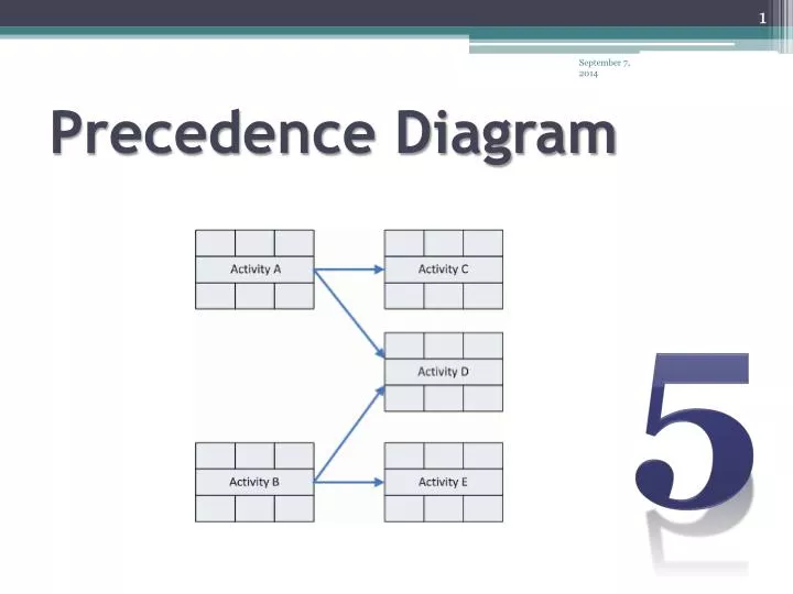
Precedence Diagram. 5. The Four Types Relationships. Activities represented by nodes and links that allow the use of four relationships: 1) Finish to Start – FS 2) Start to Finish – SF 3) Finish to Finish – FF 4) Start to Start – SS.

E N D
The Four Types Relationships • Activities represented by nodes and links that allow the use of four relationships: 1) Finish to Start – FS 2) Start to Finish – SF 3) Finish to Finish – FF 4) Start to Start – SS
Finish to Start (FS) Relationship . The traditional relationship between activities. . Implies that the preceding activity must finish before the succeeding activities can start. . Example: the plaster must be finished before the tile can start. Plaster Tile
Star to Finish (SF) Relationship . Appear illogical or irrational. . Typically used with delay time OR LAG. . The following examples proofs that its logical: if I start ordering concrete I can finish pouring. Can I finish pouring without ordering? Erect formwork steel reinforcement Pour concrete 5 SF Order concrete
Finish to Finish (FF) Relationship • Both activities must finish at the same time. • Can be used where activities can overlap to a certain limit. Erect scaffolding Remove Old paint FF/1 sanding FF/2 Dismantle scaffolding painting inspect
Start to Start (SS) Relationship • This method is uncommon and rarely exists in project construction . Clean surface Spread grout SS Set tile Clean floor area
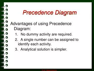
Advantages of using Precedence Diagram • No dummy activities are required. • A single number can be assigned to identify each activity. • 3. Analytical solution is simpler.
Calculation • forward calculations • EF = ES + D • Calculate the Lag • LAGAB = ESB – EFA • Calculate the Free Float • FF = Min. (LAG)
2) Backward calculations For the last task LF=EF , if no information deny that. LS=LF-D Calculate Total Float TF = LS – ES OR LF – EF TFi = Min (lag ij + TFj ) Determine the Critical Path
Example 1) Forward pass calculations 4) Backward pass calculations 5) Calculate total Float (TF = LS – ES OR LF – EF) B D F H A 0 0 0 0 1 2 11 16 20 1 1 9 2 5 11 4 16 1 20 0 0 2 0 0 11 0 0 16 0 0 20 0 0 21 2 11 16 20 21 4 5 3 0 G C E 0 0 2 7 11 5 5 4 10 6 14 0 3 10 0 3 14 3 3 20 7 11 17 2) Calculate the Lag ( LAGAB = ESB – EFA) ES Dur. LS 3) Calculate the Free Float (FF) FF = min.( LAG) EF FF TF LF 10
6) Determine the Critical Path A B D F H 0 0 0 0 1 2 11 16 20 1 1 9 2 5 11 4 16 1 20 0 0 2 0 0 11 0 0 16 0 0 20 0 0 21 2 11 16 20 21 4 5 3 0 G C E 0 0 2 7 11 5 5 4 10 6 14 0 3 10 0 3 14 3 3 20 7 11 17 ES Dur. LS The critical path passes through the critical activities where TF = 0 EF FF TF LF 11
CATEGORIES OF RESOURCES • Labor • Materials • Equipment’s.
Labor 1. Salaried staff: like-project engineer, secretary. 2. Hourly workers: like-carpenters. Equipment and Materials 1. Construction equipment and materials 2. Installed equipment and materials
What is resource allocation? Resource allocation(resource loading) : Is the assignment of the required resources to each activity, in the required amount and timing. What Is Resource Leveling? Is minimizing the fluctuations in day-to-day resource use throughout the project. It is usually done by shifting noncritical activities within their available float. It attempts to make the daily use of a certain resource as uniform as possible.
Why level Resources? 1. When the contractor adds the daily total demand for a specific resource for all activities he must provide the required amount, or work will be delayed. 2. Leveling may also be necessary for an expensive piece of equipment. 3. The main idea of resource leveling is to improvework efficiencyand minimize costduring the life of the project. Note: In general, materials do not need to be leveled
Leveling Resources in a Project • Resource leveling is a mathematically complex process. • The resource-leveling method is called the minimum moment algorithm. • discussed by Robert B. Harris (1978) in his classic textbook, Precedence and Arrow Networking Techniques for Construction
Resource Profiles Resource need Actual, not leveled Leveled, realistic Ideal Time
Sort Sort : the process of arranging activities in a list to certain specific order.
Priorities & Sorts • The activities making up the network must be listed in order of their priority of resources allocation. • The network shows the logical sequence of activities. (predecessor and successor). • The listing of activities must therefore reflects the dependency of some activities .
Activities Sort Activity sort reflects the logic sequence of the network.
Major Sort Activity sort with ES time as Major sort
Major & Minor Sorts Activity sort with ES time as Major sort & TF as Minor Sort
Allocated resources 8H A 9H 9H 9H 9H 9H 9H 9H 9H 9H B 7H 7H 7H 7H 7H C Activity 4H 4H 4H 4H E 5H 5H 5H 5H 5H D 2H 2H 2H 2H 2H 2H G 8H 8H 8H 8H F 4H H 2 4 6 12 8 10 14 16 18 20 Time
Time 2 4 6 12 8 10 14 16 18 20 8H A 9H 9H 9H 9H 9H 9H 9H 9H 9H B 7H 7H 7H 7H 7H C 4H 4H 4H 4H E Activity 5H 5H 5H 5H 5H D 2H 2H 2H 2H 2H 2H G 8H 8H 8H 8H F 4H H 8 16 16 16 16 16 13 13 13 13 7 7 7 7 7 10 8 8 8 4 Total Labor Early start resources aggregation
Resource Aggregation Resources aggregation: is a summation of the resources that are used to carry out the program on a time period basis. For example, day to day , or week to week.
4 8 16 16 16 16 16 13 13 13 13 7 7 7 7 7 10 8 8 8 Total Labor 16 14 Labor 12 10 8 6 4 2 2 4 6 12 8 10 14 16 18 20 27 Time Early start resources aggregation diagram (Histogram)
Late start • Another histogram can be obtained if Late start considered. Shows different resources demand. • And many histograms can be obtained considering a different time in the network. • Each histogram shows different resources demand.
late Start Sorts Activity sort with LS time as Major sort & TF as Minor Sort
Time 2 4 6 12 8 10 14 16 18 20 8H A 9H 9H 9H 9H 9H 9H 9H 9H 9H B 7H 7H 7H 7H 7H C 4H 4H 4H 4H E Activity 5H 5H 5H 5H 5H D 2H 2H 2H 2H 2H 2H G 8H 8H 8H 8H F 4H H 8 9 9 9 16 16 16 16 16 13 9 9 9 7 7 10 10 10 10 4 Total Labor Late start resources aggregation
8 9 9 9 16 16 16 16 16 13 9 9 9 7 7 10 10 10 10 4 Total Labor 16 14 Labor 12 10 8 6 4 2 2 4 6 12 8 10 14 16 18 20 Time Late start resources aggregation diagram (Histogram)
8 9 9 9 16 16 16 16 16 13 9 9 9 7 7 10 10 10 10 4 Total Labor 16 14 Labor 12 10 8 6 4 2 2 4 6 12 8 10 14 16 18 20 Time 32 Early start vs Late start resources aggregation diagram (Histogram)
8 9 9 9 16 16 16 16 16 13 9 9 9 7 7 10 10 10 10 4 Total Labor 16 14 Labor 12 10 8 6 4 2 2 4 6 12 8 10 14 16 18 20 Time 33 Early start vs Late start resources aggregation diagram (Histogram)
E Example 10 6 16 6 22 16 6 B F I 6 11 13 12 17 19 3 4 2 6 16 6 19 6 22 10 0 13 0 16 6 A C G K 11 22 11 22 1 5 5 2 3 1 6 6 0 14 0 24 0 6 14 0 24 0 0 11 6 0 11 0 D J 6 12 2 14 14 8 6 14 8 0 0 22 22 0 H ES Dur. LS 8 EF LF 16 6 FF TF 8 22 14 8
Activities Sort Activity sort with ES time as Major sort & TF and duration as Minor Sorts
Time 2 22 4 6 12 24 8 10 14 16 18 20 8H 8H 8H A 8H 8H C 2H 2H 2H 2H 2H D 4H 4H B 9H 9H 9H 9H 9H 9H 9H 9H H 5H 5H 5H 5H 5H 5H E 5H 5H 5H 5H 5H 5H G 2H 2H 2H F 8H 8H I 5H 5H 5H J 2H 2H 2H 2H 2H 2H 2H 2H 6H K 6H Total Labor 8 8 8 8 8 15 15 16 16 12 20 20 17 12 12 2 2 2 2 2 2 6 6 Early start resources aggregation
Total Labor 8 8 8 8 8 15 15 16 16 12 20 20 17 12 12 2 2 2 2 2 2 6 6 20 18 16 14 Labor 12 10 8 6 4 2 2 22 4 6 12 24 8 10 14 16 18 20 Early start resources aggregation diagram Time
Activities Sort Activity sort with LS time as Major sort & TF and duration as Minor Sorts
Time 2 22 4 6 12 24 8 10 14 16 18 20 8H 8H 8H A 8H 8H C 2H 2H 2H 2H 2H D 4H 4H B 9H 9H 9H 9H E 5H 5H 5H 5H 5H 5H H 5H 5H 5H 5H 5H 5H G 2H 2H 2H F 8H 8H I 5H 5H 5H J 2H 2H 2H 2H 2H 2H 2H 2H 6H K 6H Total Labor 8 8 8 8 8 2 2 2 2 2 2 15 15 11 11 12 20 20 17 17 17 6 6 Late start resources aggregation
Total Labor 8 8 8 8 8 2 2 2 2 2 2 15 15 11 11 12 20 20 17 17 17 6 6 20 18 16 14 Labor 12 10 8 6 4 2 2 22 4 6 12 24 8 10 14 16 18 20 Late start resources aggregation diagram Time
20 20 18 18 16 16 Labor Labor 14 14 12 12 10 10 8 8 6 6 4 4 2 2 Early start Late start
Smoothing/Leveling • Let us program activity F to start by its late start day which is day 17. • And activity I to start by day 14. • The resulting resources aggregation histogram will be as follows:
Time 2 22 4 6 12 24 8 10 14 16 18 20 8H 8H 8H A 8H 8H C 2H 2H 2H 2H 2H D 4H 4H B 9H 9H 9H 9H 9H 9H 9H 9H H 5H 5H 5H 5H 5H 5H E 5H 5H 5H 5H 5H 5H G 2H 2H 2H F 8H 8H I 5H 5H 5H J 2H 2H 2H 2H 2H 2H 2H 2H 6H K 6H Total Labor 8 8 8 8 8 15 15 16 16 12 12 12 12 12 12 7 10 10 2 2 2 6 6 Early start resources aggregation
Total Labor 8 8 8 8 8 15 15 16 16 12 12 12 12 12 12 7 10 10 2 2 2 6 6 20 18 16 14 Labor 12 10 8 6 4 2 2 22 4 6 12 24 8 10 14 16 18 20 Time
Smoothing/Leveling • Let us program activity E to start by its late start time. • So its resources demand starts with its Late start date. • The resulting resource aggregation and histogram will be as follows:
Time 2 22 4 6 12 24 8 10 14 16 18 20 8H 8H 8H A 8H 8H C 2H 2H 2H 2H 2H D 4H 4H B 9H 9H 9H 9H 9H 9H 9H 9H H 5H 5H 5H 5H 5H 5H E 5H 5H 5H 5H 5H 5H G 2H 2H 2H F 8H 8H I 5H 5H 5H J 2H 2H 2H 2H 2H 2H 2H 2H 6H K 6H Total Labor 8 8 8 8 8 15 15 16 16 7 15 15 12 7 7 7 7 7 7 7 7 6 6
Total Labor 8 8 8 8 8 15 15 16 16 7 15 15 12 7 7 7 7 7 7 7 7 6 6 20 18 16 14 Labor 12 10 8 6 4 2 2 22 4 6 12 24 8 10 14 16 18 20 Time
Smoothing/Leveling • In case activity D is split able activity. It could be interrupted to be carried out in tow parts. • Let us program activity B to start by 7th day . • And activity H to starts by its Late start date. • And activity E to start by day 14. • The resulting resource aggregation and histogram will be as follows:
Time 2 22 4 6 12 24 8 10 14 16 18 20 8H 8H 8H A 8H 8H C 2H 2H 2H 2H 2H D 4H 4H B 9H 9H 9H 9H H 5H 5H 5H 5H 5H 5H E 5H 5H 5H 5H 5H 5H G 2H 2H 2H F 8H 8H I 5H 5H 5H J 2H 2H 2H 2H 2H 2H 2H 2H 6H K 6H Total Labor 8 8 8 8 8 6 11 11 11 11 10 10 11 12 12 12 12 12 12 7 7 6 6 Early start resources aggregation
Total Labor 8 8 8 8 8 6 11 11 11 11 10 10 11 12 12 12 12 12 12 7 7 6 20 18 16 14 Labor 12 10 8 6 4 2 2 22 4 6 12 24 8 10 14 16 18 20 Time