3. Boundary Value Problems II

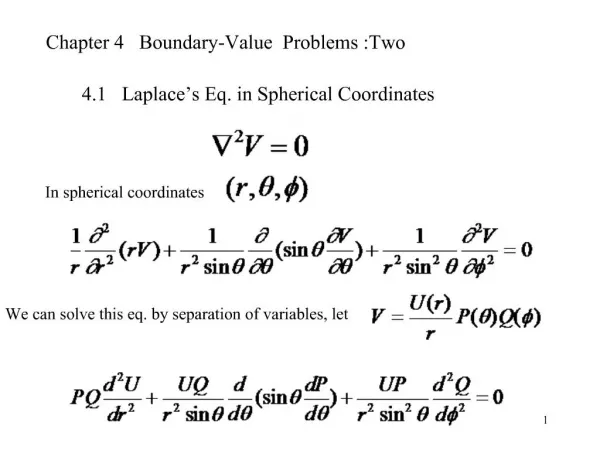
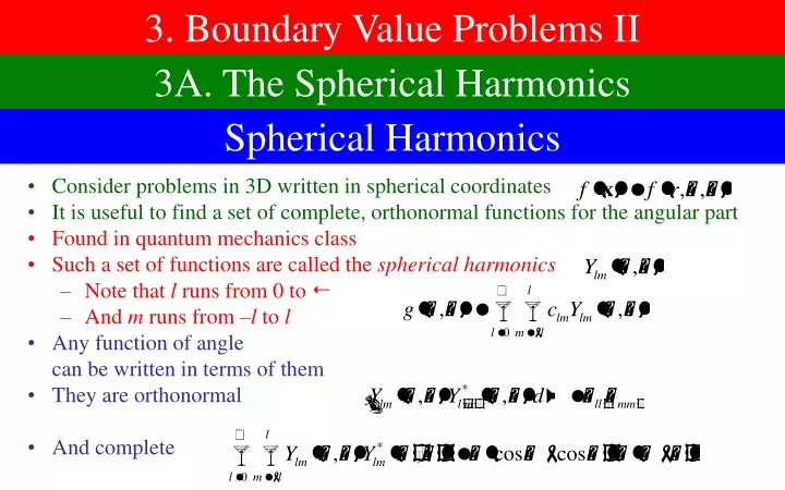
1. 3. Boundary Value Problems II 3A. The Spherical Harmonics Spherical Harmonics • Consider problems in 3D written in spherical coordinates • It is useful to find a set of complete, orthonormal functions for the angular part • Found in quantum mechanics class • Such a set of functions are called the spherical harmonics • Note that l runs from 0 to  • And m runs from –l to l • Any function of anglecan be written in terms of them • They are orthonormal • And complete

2. Properties of Spherical Harmonics •  dependence: •  dependence • Pl|m| is a polynomialof order l – |m| • Complex conjugate: • Parity: changing x  –x • In angles,    –  and   –  • Value at  = 0: • Explicit form can be found in many sources • Look them up, use Maple program, or do whatever is most useful to you

3. The Spherical Harmonics

4. Spherical Harmonics and Legendre Functions • Legendre functions are a set of n’th order polynomials • They are orthogonal on the interval (–1, 1) • They are “normalized” by the condition • Compare to the normalization condition • Recall these functions have no  dependence • Recall that Yl0 is an l’th order polynomial in cos • It is clear that Yl0 and Plare almost the same thing

5. Spherical Harmonics and the Laplacian • Spherical harmonics satisfy • Compare to the Laplacian • Suppose we write afunction in the form: • Then the Laplacian acting on this will give

6. Problems with No Charge in a Region • Suppose we have no charge in a region, so • Then we must have: • Need two independent solutions, since 2nd order differential equation • Let’s try clm ~ r • Solutions are  = l or  = –l– 1 • Therefore • If we want finite at 0, don’t include B • If we want zero at , don’t include A

7. Spheres with Boundary Conditions • Suppose we have a sphere, radius a, potential given on surface • We want potential inside or outside • The general solution inside will be • Match at r = a: • To find coefficients, multiply by Yl'm'* and integrate over angles • So we have: • Similarly:

8. Sample Problem 2.3 Redux The potential on the surface of a sphere of radius a centered at the origin is given by  = Ez. Find the potential outside the sphere. x z • Write potential as • We then note • So we have • Our answer is • Where • So we have

9. Sample Problem 3.1 (1) The potential on the surface of a sphere of radius a centered at the origin is given by  = V for cos > 0 and  = –Vfor cos < 0 Find the potential outside the sphere. • Our answer is • Where • Recall that • Integral vanishes unless m = 0 • Parity tells you • Only odd l contributes, for which

10. Sample Problem 3.1 (2) The potential on the surface of a sphere of radius a centered at the origin is given by  = V for cos > 0 and  = –Vfor cos < 0 Find the potential outside the sphere. • If needed, that last integral can actually be done in closed form • Put it all together • For r/a large, terms rapidly converge

11. 3B. The Free Green’s Function Setting it up • Dirac delta in 3D inspherical coordinates: • You can tell this is right, because: • The Green’s function in free space satisfies: • Use completeness to write right hand side in terms of spherical harmonics

12. Factoring G into Radial and Angular Functions • The Green’s function, like anyfunction, can be written in the form • When we put thisin the Laplacian,we get • Matching this withabove, we have • We know solution whenright side vanishes for r  r' • To make it finite at r = 0and at r = , must have

13. Factoring G into Radial and Angular Functions • The Green’s function, like anyfunction, can be written in the form • When we put thisin the Laplacian,we get • Matching this withabove, we have • We know solution whenright side vanishes for r  r' • To make it finite at r = 0and at r = , must have

14. Matching at the Boundary • Multiply this by r, then integrate from r = r' –  to r = r' + , where  is small • First term integrated by fundamental theorem of calculus • Second term is small • Right side is trivial • Substitute in: • Since finite discontinuity inderivative, function must be continuous

15. Putting it All Together • Substitute the secondformula in the first: • We therefore have have • In summary,

16. Multipole Expansion • Green’s functions are used to calculate thepotential from an arbitrary charge distribution • For example, let’s find the potential outside a localized distribution • So r > r' • Define the multipole moments ofthe distribution qlm by the expression • Note that it iseasy to show that • Then the potential is given by • Leading terms are large rare given by small l

17. Sample Problem 3.2 (1) A localized charge distribution takes the form . Find the first two non-vanishing contributions to the multipole expansion, and the potential at large r. • The multipole moments are: • In sphericalcoordinates: • Recall that • Integral vanishes unless m = 0, in which case the  integral just yields 2 • Parity can be used to argue that the  integral vanishes unless l is odd • Radial integral can be done explicitly: • So we have: • There’s a reasonwe have Maple: > for l from 1 to 11 by 2 do integrate(spherharm(l,0)* sin(theta)*(Pi/2-theta),theta=0..Pi) end do;

18. Sample Problem 3.2 (2) A localized charge distribution takes the form . Find the first two non-vanishing contributions to the multipole expansion, and the potential at large r. • We find • The potential is given by • If you prefer,

19. Green’s Function Inside a Sphere • Suppose we had a grounded conducting hollow sphere with charge inside • We already know the Green’sfunction(from method of images): • First term we alreadyknow how to write: • For the second term, multiply by a/r and replace r by a2/r • Note that a2/ris always larger than r', so we have • Put it together:

20. Sample Problem 3.3 (1) A hollow conducting sphere of radius a has a line charge  along the z-axis. Find the potential everywhere • This is tricky, since the line charge is at  = 0 and  =  • The value of  is irrelevant, since we are on the z-axis • We want the charge density to integrate to 2a • In spherical coordinates, we would have • Check it: • Now use the Green’s function:

21. Sample Problem 3.3 (2) A hollow conducting sphere of radius a has a line charge  along the z-axis. Find the potential everywhere • Work on everything in the blue box • Only even l contribute

22. Sample Problem 3.3 (3) A hollow conducting sphere of radius a has a line charge  along the z-axis. Find the potential everywhere • So final answer is:

23. 3C. Green’s Function in a Box Using a Complete Set of Modes • Green’s Function for a 3d box of dimensions a  b c • Green’s function must satisfy • And must also satisfy • Any function thatvanishes on boundarymust take the form • The same withdeltafunction • Substitute into our equation: • Since our functions are independent:

24. Finding the Green’s Function • We can find the B’s using the orthonormality of the sine functions • Put it all together and we have the Green’s functions:

25. Sample Problem 3.4 A cubical box of side a has potential zero on the surface and a surface charge density  at z = a/2. Find the potential everywhere. • Charge density is • Potential is

26. Sample Problem 3.5 A cubical box of side a has potential zero on the surface and uniform charge  inside. Find the potential everywhere. • Potential is

27. 3D. Solving Problems in a Cylinder Azimuthal Dependance • For problems in cylinders, we will work in cylindrical coordinates • Write functions as • Laplacian in cylindrical coordinates: • Helpful to have complete orthonormal functions for these variables • For : it is naturally periodic, since  = 0 is the same as  = 2 • We know a complete set of functions like this: • These are complete and (almost) orthonormal: • They are alsonice because • Any function of  can be written in terms of these • The constants fm can be found from • Can also use functions

28. Z - Dependance • We might also need some complete functions in the z-direction • If there is no restriction on z, this might be • Complete and almost orthonormal • These are also helpful because • If instead, we have a problem where function vanishes atz = 0 and z = c, then we can use as our complete functions • Again, almost orthonormal • This leaves us to find “nice” basis of functions for  dependence

29. Bessel Functions • Let’s try to find functions R()that satisfy the equation • Divide this equation by k2 • Define a new variable • Then • This is called Bessel’s Equation • For each value of m, two linearlyindependent solutions: • J is called a Bessel function and N is called a Neumann function • General solution of originalequation is therefore

30. Properties of Bessel Functions • Nice series expression for the Bessel functions: • The Jm’’s are well behaved at theorigin, the Nm’s are not • At large x, they oscillate • They have aninfinite number of roots • Maple is happy to compute the functions • Maple can also find roots for you > BesselJ(m,x);BesselY(m,x) > BesselJZeros(m,n);

31. Bessel Functions With Boundary Conditions • Our Bessel functions satisfy: • If we want them to be well-behaved atthe origin, only want to use Jm’s • If it is forced to vanish at some radius a, then • We know the roots of Jm are xmn, so • We therefore want to write functionsof  in terms of these functions: • Are these functions orthogonal? • Not terribly hard to show that this vanishes unless n = n' • Harder to actually find the integral

32. Bessel Functions Are Complete and Orthogonal • Given any function on a circle, we write it in polar coordinates: • We then write this function in terms of the azimuthal modes: • If the function vanishes at  = a, we expand the g’s in terms of Bessel functions • We can always findthe coefficients Amn:

33. Cylinder with Ends Specified (1) • Consider a cylinder radius a and height c with no charge inside • Potential is zero on lateral surface, specified on top and bottom • We write the potential everywhere in the form • Substitute intoLaplace’s equation: • Bessel functions satisfy Bessel’s equation: • Therefore:

34. Cylinder with Ends Specified (2) • Only way this canbe satisfied is if • General solutionof this equation is • So we have: • Must still match on thebottom and the top

35. Matching the End Conditions • We can use orthogonality to get the coefficients for the bottom • Look back three slides • In a similar manner, for the top we have • Two equation in two unknowns • Solve for mnand mn and substitute in

36. Sample Problem 3.4 (1) A cylinder of radius a and height 2a has potential  = 0 on the lateral boundary and  = V on the ends. Find the potential everywhere, and particularly at the center • Center at origin • Potential is • On the ends,this implies • Use ortho-gonalityto find • Subtract thetwo equations: • Therefore:

37. Sample Problem 3.4 (2) A cylinder of radius a and height 2a has potential  = 0 on the lateral boundary and  = V on the ends. Find the potential everywhere, and particularly at the center • The  integral is zero unless m = 0 • For final integral,let y = /a • Make Maple do the work > for i to 10 do evalf(2*int(y*BesselJ(0,BesselJZeros(0,i)*y), y=0..1)/BesselJ(1,BesselJZeros(0,i))^2) end do;

38. Sample Problem 3.4 (3) A cylinder of radius a and height 2a has potential  = 0 on the lateral boundary and  = V on the ends. Find the potential everywhere, and particularly at the center • To get the value at the origin, set z = 0 and  = 0 • J0(0) = 1 and cosh(0) = 1 • Add seven terms

39. Cylinder with Lateral Surface Specified • What if the potential were specified on the sides instead? • We want complete functions that vanish on z = 0 and z = c • And still periodic on  • This suggests using modes • Write a complete set of functions • Substitute intoLaplace’s equation • Since these are completeorthonormal functions on and z, we must have

40. Modified Bessel Functions • Almost like Bessel’s Equation but sign on last term is wrong sign • The solutions are actually modified Bessel functions • They are essentially Bessel functions with imaginary arguments • The Km’s diverge at the origin, so don’t use them • It then has to matchon the boundary  = a • Orthogonality letsyou find the A’s

41. Sample Problem 3.5 (1) A cylinder of radius a and height 2a has potential  = 0 on the top and bottom and  = V on the lateral surface. Find the potential everywhere, and particularly at the center • Bottom at z = 0 • Potential is • On the lateral surface • Use orthogonalityto find • Therefore:

42. Sample Problem 3.5 (2) A cylinder of radius a and height 2a has potential  = 0 on the top and bottom and  = V on the lateral surface. Find the potential everywhere, and particularly at the center • At center,we have • I0(0) = 1, andsine alternates • Let Maple do the work > add(4*evalf((-1)^n/BesselI(0,Pi*(n+1/2))/(2*n+1)/Pi),n=0..6);

43. Sample Problem 3.5b A cylinder of radius a and height 2a has potential  = V on all surfaces. Find the potential at the center The hard way • We previously solved it forjust the ends or just the sides: • By superposition, the potentialfor this problem is the sum of these two problems The easy way: • The solution of Poisson’s equation is: • Sometimes, clever approaches can give you the answer much more quickly • You could have done the first problem by subtraction