Download
1 / 23
230 likes | 241 Views
EART10160 stats / data analysis descriptive stats and outliers. Dr Paul Connolly. Next 5 weeks. I will talk around the relevant science / maths in the lecture See webpage for material I will introduce the practical We will then go to computers: Log on to Blackboard

E N D
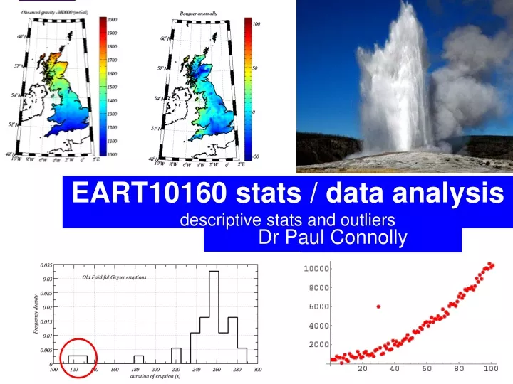
EART10160 stats / data analysisdescriptive stats and outliers Dr Paul Connolly
Next 5 weeks • I will talk around the relevant science / maths in the lecture • See webpage for material • I will introduce the practical • We will then go to computers: • Log on to Blackboard • start the practical exercises • Demonstrators will help with questions (but not give answers) • You can use MS Excel / MATLAB to do the exercises, why?
Frequency tables and histograms • This week I would like you to generate a histogram of data, and calculate some basic stats • A frequency histogram is a plot of binned data using the bin mid-points and the frequency in the bin as x and y values respectively. • Excel doesn’t do this by default… • It uses upper bin edges. • So bin upper edges need to be shifted before plotted
Overview this week • Descriptive statistics (4 slides of definitions!): • Mean, Median, Mode • Standard deviation, variance, standard error, range. • Outliers: • Spotting them in histograms • Definition using `z-score’ • Rare values: • Determined using `z-score’ • Visual comparison of histograms
Definition: Mean, page 8 notes • xi= values in a list • - means to sum all values N = number of data points in a list (sample size). Excel: =AVERAGE(A1:A10) (see table page 45 of notes) MATLAB: mean(dat) (see table page 45 of notes)
Definition: Median and Mode • Median: half way point in a ranked list of numbers. • Excel: `=median(A1:A10)’(see table page 45 of notes) • MATLAB: `median(dat)’(see table page 45 of notes) • Mode: most frequent value (the highest point in a histogram) • Excel: `=mode(A1:A10)’(see table page 45 of notes) • MATLAB: `mode(dat)’(see table page 45 of notes)
Definition: Standard deviation, page 9 notes • xi= values in a list • - means to sum all values N = number of data points in a list. For normally distributed data: 68.3% of data lies within 1 standard deviation of the mean 95.5% of data lies within 2 “ 99.9% of data lies within 3 “ Excel `=STDEV(A1:A10)’ (see table page 45 of notes) MATLAB `std(dat)’ (see table page 45 of notes)
Definition: z-score If you don’t know the population mean,, just use the sample mean. This tells us how many standard deviations away from the mean a value is. Remember that for normally distributed data: 68.3% of data lies within 1 standard deviation of the mean 95.5% of data lies within 2 “ 99.9% of data lies within 3 “
See OLDFAITH.xls Duration of eruption
Frequency histogram • Frequency histogram: binned data
Frequency density: • Frequency divided by the sum of the total, divided by the bin width • Area under the curve=1 • Cumulative Frequency: • Cumulative sum of frequency histogram (from the left) divided by the total. • Max value of curve=1 What value is 90% of the data less than (or 10% of the data larger than)?
Page 29 says The wording is atrocious! (and probably purposely written so that lay people do not understand it.) In other words, just produce a cumulative frequency plot and find the sound level corresponding to cumulative frequency=0.9
How do we quantitatively say that these are unusual? How can we tell whether the duration of eruptions of old faithful is changing or unusual? • The histogram is asymmetric • Visually, they are separated from the main `mode’ • Could also calculate the z-score for the list of data.
Key Point:Rare values are not the same as outliers, but statistically can be determined in a similar way (e.g. calculating the z-score)…
Geophysics: gravity anomalies • Gravity: more mass = higher attraction. • BGS measure the observed gravity in units of mGal (1x10⁻⁵ m s-2) • Tell you about the geology of the UK.
Histogram of observed gravity over the UK • The positive skew makes observed gravity difficult to analyse statistically. Positively skewed i.e. every so often it is higher than most of the values
Geophysics: the Bouguer anomaly • Difference between expected value of gravity and actual. • +ve anomaly means there is less gravity than expected • and vice-versa. • Tells you about how dense the underlying surface is. • i.e. if there is a large oil field or meteorite below the surface.
It turns out that distribution Bouguer anomaly over the UK almost symmetrical. It is normally distributed this makes it much easier to analyse in the context of this course (next practical). There are no obvious outliers in the histogram. Although there are no obvious outliers, you will be asked whether a value is unusual. In this context we are asking whether a value is rare: z-score
Either do in Excel or MATLAB (help will be on hand) • YouTube tutorials • Spreadsheets and data.
MATLABers, if you want to learn how to plot out the landgrav data from BGS see second page • `scatter’ function deals with ungridded 2-d spatial data • We will also learn how to deal with gridded data. • I would not know how to do this in Excel.
Week 7 practical • You are given several datasets and asked to say whether different values are usual or un-usual. • Use the z-score to say how many standard deviations from the mean the values are. Larger than 2 standard deviations are un-usual. • You are asked to look at a cumulative frequency distribution and comment on it. • You are asked to create several histograms – practice, practice, practice. • You are asked to compare different histograms of VOLTAGES to say whether different datasets are different. • Look to see how much of the histograms over-lap with each other and how different the modes, and variations are.