Download
1 / 17
170 likes | 241 Views
HMM in crosses and small pedigrees, cont. Lecture 9, Statistics 246, February 19, 2004. Another problem: reconstructing haplotypes. The problem here is to reconstruct the childrens’ haplotypes as in the figure, from marker data on both the children and the parents. The Lander-Green HMM.

E N D
HMM in crosses and small pedigrees, cont. Lecture 9, Statistics 246, February 19, 2004
Another problem: reconstructing haplotypes The problem here is to reconstruct the childrens’ haplotypes as in the figure, from marker data on both the children and the parents.
The Lander-Green HMM • Recap. The states of the Markov chain are the inheritance vectors. At any locus on a chromosome, the entry in the inheritance vector for a non-founder are 0 if the parental variant passed on at that locus was grandmaternal, and 1 otherwise. • Consider a two-parent two-child nuclear family and suppose that the mother and father are 1/2 and 3/4, respectively, while the first (girl) child is 1/3 and the second (boy) is 2/4. Then the inheritance vector is of length 4, v = (vgm , vgp , vbm, vbp), where gm represents the girl’s maternal meiosis, gp her paternal meiosis, and so on. • What are the assigments for v at the marker? We don’t know which of the mother’s alleles 1 and 2 came from her mother and which came from her father, but we can arbitrarily declare that it was the one she passed on to her daughter, and similarly for the alleles 3 and 4 of the father. With this assignment, we find that v = (0, 0, 1, 1), because in each case, the boy received alleles from his parents different from his sister’s. In fact the specification of the paternal and maternal chromosomes of a founder is completely arbitrary, and we’ll mention later how this can be turned into a symmetry which speeds up the calculations.
Transition probabilities • Now suppose that the same family has genotypes 1’/2’, 3’/4’, 1’/3’ and 2’/4’ at a locus near the first one. If the recombination fraction between the two loci is r, and r is small, then we might expect the inheritance vector v’ at the second locus to coincide with v = (0,0,1,1). But what if the genotypes were 1’/2’, 3’/4’,1’/3’ and 2’/3’, respectively? This suggests that v’ = (0,0,1,0), with the 10 in the boy’s paternally inherited chromosome denoting a recombination. • How do we weigh up these competing possibilities? As with the mouse chromosomes, we need a transition matrix P(r) connecting adjacent inheritance vectors. The form of P is as in the mouse case, namely, a tensor power of the 22 matrices having 1-r on the diagonal, and ron the off-diagonal elements, here P = R(r)4 . In general, it is an 2nth tensor power, where n is the number of non-founders. Thus we have our states and our transition probability matrix, and hence our (product) Markov chain. • To complete the specification of our HMM, we need observations and the associated emission probabilities, and an initial distribution.
Alternative representation • The purpose of inheritance vectors is to describe the possible patterns of gene flow through a pedigree. Once ordered pairs of alleles are assigned to founders, the 0s and 1s in the inheritance vectors specify the alleles that are passed from parent to offspring down the pedigree. As mentioned in the last lecture, an alternative representation of this gene flow is via what is known as a descent graph, see Lange’s book, ch 9. • A recent paper gave an even more economical representation of what is needed, via what the authors called a sparse gene flow tree. I leave those interested to consult Abecasis et al, Nature Genetics 302002: 97-101. • There (in the program Allegro) the efficient matrix multiplication that we will describe shortly is replaced by a sparse matrix-vector multiplication algorithm more general that the one we will give.
Observations (phenotypes) • We now turn to our observations. The data we have on our (small) pedigree will generally consist of genotypes at many marker loci, and perhaps additional disease or other phenotype data, see the pedigree on p.2, where black filling of a square or circle indicated that the person is affected by some specified disease. In the case of interest to us here: reconstructing haplotypes, we’ll assume that there are just marker data. • Suppose the unordered pairs of alleles (i.e. genotypes) at marker locus t come from a set (t). Then for f founders and n non-founders, our observations come from (t)f(t)n. Here I could have simply written the (f+n)th power, but it is convenient to keep founders and non-founders notationally distinct. As with the mouse crosses, we could add in ambiguity and missing data “observations”, but for simplicity we won’t do so here. Since we are mainly interested in marker data, let’s denote a typical (vector) observation at locus t by mt.
Emission probabilities • Referring to our general discussion of HMM in the previous lecture, we now need to specify the equivalent of the emission probabilitiesq(i,j,k; t) at each locus t. These probabilities are generally functions of the current and previous state, but here they just depend on the current state, vt , and take the form q(vt ,mt ; t). We want this to be • q(vt ,mt ; t) = pr(observations at t = mt | inheritance vector at t =vt ), • but right now vt just describes gene flow: we haven’t got started. • To complete our description, let us write at = (at,1 ,at,2 ….,at, 2f-1 ,at, 2f ) for the assignment of an ordered pair of alleles to each founder. Suppose that the frequency of allele at,h is pt,h . Under the population equilibrium assumptions we have previously mentioned, pr(at ) =∏h pt,h . Finally, we sum over all at (in practice, over all at compatible with the observed phenotypes). This gets us started towards defining q(vt ,mt ; t).
Penetrances • Having got started, note that alleles at for the founders and an inheritance vector vt gives us a set of orderedgenotypes gt = (at ,vt ) at locus t by following the flow. We are almost there. • The observations on each individual in the pedigree can now be assigned probabilities given their (ordered) genotypes. This last step involves the terms we have previously called penetrances - probabilities of observed phenotypes given genotypes - and a non-trivial assumption: that the probabilities of the different individuals’ phenotypes are conditionally independent given their (ordered) genotypes, and depend on the pedigree’s (ordered) genotypes only on their own (ordered) genotypes, • i.e. pr(mt | gt ) = ∏ipr(mt,i | gt,i ), • where the product is over individuals i in the pedigree, and the terms in the product are penetrances. • Putting all this together, our HMM emission probabilities have the form • q(vt ,mt ; t) = ∑ pr(at )pr(mt | at ,vt ) = ∑ ∏ pt,h ∏ipr(mt,i | gt,i ).
Pedigree calculations • The HMM is fully specified as soon as we give an initial distribution for the states, and this is simply the uniform distribution: each inheritance vector is assigned initial probability 2-2n. • We now turn to carrying out the calculations efficiently, so that we can deal with as large small pedigrees as possible. Since the HMM formulation of pedigree analysis was introduced by Lander and Green in 1987, there have been a number of improvements. Looking back over nearly 20 years of these, the arms race comes to mind. Details of the first human version Crimap were never published, but it would have used the standard HMM simplifications we will review shortly. In 1995 Genehunter came on the scene, Kruglyak et al (1995,1996), and this had a few new tricks. Then Genehunter+ incorporated founder phase symmetry and what Kruglyak and Lander (1998) called Fourier analysis (on {0,1}n). The next improvement was Allegro (Gudbjartsson et al 2000), whose tricks are yet to be revealed to the world, and the most recent and fastest is Merlin (Abecasis et al, 2002), which uses sparse gene flow trees and some ideas from coding theory. The race will go on!
The forward equations • It is time to present the standard HMM formulae, these going back to the original work of Baum et al, c1970. We will revert to the general HMM notation for this discussion, that is, our HMM has components (Xt, Yt), with Xt “hidden” and Yt observed. With Baum et al, define the forward quantities 1(i) = pr(Y1,X1 = i), where i is an arbitrary state of X1 , and • t+1(j) = pr(Y1,Y2,…..,Yt+1 , Xt+1 = j) • = ∑ipr(Y1,Y2,…,Yt ,Yt+1 , Xt = i, Xt+1 = i) • = ∑i pr(Y1,Y2,…,Yt , Xt = i) pr(Xt+1 = j |Y1,Y2,…Yt , Xt = i) • pr(Yt+1 |Y1,Y2,…,Yt , Xt = i, Xt+1 = j ) • = ∑it(i)p(i, j; t)q(i, j,Yt+1; t+1). • When these are all computed up to T, simply sum overstates i of XT to get • pr(Y1,Y2,….., YT) = ∑iT(i). • The work is in evaluating the sum, and the q terms. We look at the sum first.
Evaluating the sum (a) • In our small pedigree problem, T is the number of marker loci along our chromosome, which might be anything from 20 to 1,000, and the transition probability matrices pare all 2n2n, wheren is the number of non-founders. For small small pedigrees, such as our nuclear family, this is not a problem, but as we try to push the limits of this algorithm, the evaluation of products of such matrices by conformal vectors (which is what our sum is) becomes limiting. • How can we speed up the calculation of such products? It has been known for decades, perhaps centuries, that the application of NN matrices which are (equivalent to) tensor powers to N1 vectors can have the O(N2) multiplications reduced to O(N logN). I say centuries because it is said that Gauss used a form of the fast Fourier transform (FFT), and all these speed-ups are similar in spirit to the famous (and many times discovered) FFT. In our 2n2ncase, the speed-up goes back to Yates in the 1930s, who used it to carry out the calculations for 2nfactorial experiments. The details are in my class notes Stat 260, Week 8, Appendix to the Tuesday lecture.
Evaluating the sum (b) • The other term needing attention in the sum is the emission probability q(vt, mt; t), which we have defined as a potentially large sum over ordered pairs of alleles for all founders. A lot of effort has been devoted to finding ways of reducing the calculations • To be completed
The backward equations • In a manner quite analogous to that which gave us the forward equations, we can define T (i) = 1, and • t-1 (i) = pr(Yt,Yt+1,…..,YT | Xt-1 = i), and find that it reduces to • = ∑j t(j)p(i, j; t-1)q(i, j,Yt; t). • Exercise: Prove this. • Note that Y = (Y1,Y2,…..,YT ), then pr(Y, Xt = i) = t(i)t(i), and hence pr(Y) = ∑i t(i)t(i) for any i. • Exercise: Prove that pr (Xt = i | Y) = t(i)t(i) / ∑i t(i)t(i) , and that • pr(Xt+1 = j | Xt = i, Y) = p(i, j ; t )q(i, j, Yt+1; t+1)t+1(j) / t(i) . • Exercise:
Reconstructing the haplotypes • At last we come to our initial problem. • To be completed….
Founders: individuals without parents in the pedigree. • Non-founders: individuals with one or more parent in the pedigree
Founders: individuals without parents in the pedigree. • Non-founders: individuals with one or more parent in the pedigree
Founders: individuals without parents in the pedigree. • Non-founders: individuals with one or more parent in the pedigree