Download
1 / 38
400 likes | 641 Views
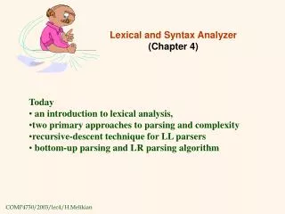
Lexical and Syntax Analyzer (Chapter 4). Today an introduction to lexical analysis, two primary approaches to parsing and complexity recursive-descent technique for LL parsers bottom-up parsing and LR parsing algorithm. Introduction.

E N D
Lexical and Syntax Analyzer(Chapter 4) • Today • an introduction to lexical analysis, • two primary approaches to parsing and complexity • recursive-descent technique for LL parsers • bottom-up parsing and LR parsing algorithm
Introduction Three different approaches to implementing languages are 1.compilation ( C++, COBOL, ADA) 2 pure interpretation (JavaScript, UNIX shell scripts, Lisp ) 3.hybrid implementation (Java, Perl) • Syntax analyzers: S_A (parsers) are nearly always based on formal description of the syntax of programs. • The most commonly used syntax description formalism is CFG or BNF
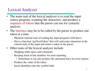
Advantages of using BNF 1. Syntax description is clear and concise for both humans and for software systems using them. 2. BNF syntax description can be used as the basis for syntax analyzer. 3.implementations based on BNF are relatively easy to maintain because of modularity. Almost all compilers separate the task of analyzing syntax into two distinct parts First: the lexical analyzer deals with small-scale language constructs as names and numeric literals Second: the syntax analyzer deals with large scale constructs, expressions, statements, and program units.
Why lexical analysis is separated from Syntax Analysis • Simplicity- lexical analysis are less complex so it is march simpler if it is separated from the syntax analyzer. • Efficiency_ it makes easier to optimize lexical analyzer and syntax analyzer. • Portability- At some point lexical analyzer is platform dependent ( remember it reads the input stream) However, the S_A can be platform independent. • It is always good idea to separate machine dependent part from the software.
Lexical Analysis Lexical analyzer is essentially a pattern matcher. The earliest uses of P_M was with text editors ( Unix ed line editor, Perl, or JavaScript). • A L_A serves as front end of S_A. Technically L_A is S_A at the lowest level of program structures. • The L_A collect characters ( from the input stream) into logical groups and assigns an internal codes to (often referenced by named construct for the sake of readability ) the groupings according to their structure. • This groupings are called lexemes . • The internal codes are called tokens.
Example sum = oldsum – value/100; token lexeme IDENT sum ASSIN_OP = IDENT aldsum SUB_OP -- IDENT value DIVIS_OP / SEMICOLON ; • L_As extracts lexemes from a given input and produce the corresponding tokens. • However, now days most L_A are subprograms • The L_A also skips comments, blanks and inserts lexemes for user-defined names into symbol table • Finally, the L_As detect syntactic errors.
Building L_A • 1.Write a formal description of the token pattern of the language using a descriptive language related to regular expressions and use a software ( special program) to automatically generate L_A. ( UNIX lexprogram • 2.Design a state transition diagram that describes the token pattern of the language and write a program that implements the diagram. • 3.Design a state transition diagram that describes the token patterns of the language and hand-construct a table driven implementation of the state diagram.
A state transition diagram • A state transition diagram , is graph like the syntax graph introduced in chapter 3. • The nodes are labeled with state names. • The arcs are labeled with the input characters that causes transitions.( it may include an actions the L_A must do when the transition is taken). • FAM as you remember can be designed to recognize a class of languages called regular languages. • Regular expressions and regular grammars are generative devices for regular languages The tokens of a programming language are regular language.
Example of L_A construction with the state diagram and the code that implements it. • The state diagram could include states and transitions for every token pattern.( it could be very large of cause). Let assume we need a L_A that only recognizes: • program names, ( strings that stars with letter followed by letter or digits no length restriction) • reserve wards ( same as names) • integer literals. ( )
First: observe that it is possible to build a state diagram to recognize every single reserve ward of language but that would result a huge state diagram. • It is much faster and easier to have the L_A recognize the names and the reserve wards with the same pattern and use lookup table of reserve wards to determine which names are reserved wards. • Second: introduce two classes of characters to simplify the state diagram: LETTER ( 52 characters) and DIGIT( 10 digits)
Next: we can define several utility subprograms for the common tasks inside the L_A 1.getChar(): gets the next character from the input and puts it in the global variable nextChar it also determines the character class of input and put it in the global variable charClass. • The lexemes being build by L_A , which could be character string or character array we name lexeme. • The subprogram addChar(); putting nextChar into the lexeme. • Finally, subprogram lookup(); to determine whether the current content of lexeme is reserve ward, or name.
lex- simple lexical analyzer int lex(){ get Char(); switch(charClass) { // parese identifiers and reserve wards case LETTER: addChar(); getChar(); while(charClass = = LETTER || charClass = = DIGIT){ addChar(); getChar(); } return looup(lexeme) break; // Parse integer literals case DIGIT: addChar(); getChar(); while( charClass = = DIGIT){ addChar(); getChar(); } return INT_LET break; } }
The Parsing Problem The part of the process of analyzing syntax that is referred to as syntax analysis S_A Is often called parser. • Next we will discuss the general parsing problems and two main categories of parsing algorithms; Top-down, Bottom-up,and also complexity of the parsing process. • Parsers, -construct parse tree for given program. In most cases information required to build parse tree is generated • There is two distinct goals of syntax analysis. • Fist : check whether or not an input program is synthetically correct. (in case of error it must produce a diagnostic message and recovery) . • Second: produce either a complete parse tree or at least trace the structure of the complete parse tree. In either cases, the result is used as the basis for translation.
Top-down and Bottom-up parsing • The parsers are categorized according to the direction in which they build parse tree. All commonly used parsing algorithms operate under the same constraint that they never look ahead more than one token into the input program. It results in elegant and efficient parsing. • Top-down- tree is build from the root downward to the leaves; In terms of derivation, the top-down parser can be describe as given a sentential form that is part of l-m-derivation the parsers task is to find the next sentential form in the lm- derivation. • Bottom-up- tree is build from the leaves upward to the root. Constructs the parse tree by the beginning at the leaves and progressing toward the root. It produces the reverse of rightmost derivation. Thus are called LR algorithms
Example : If the current sentential form is xA and A-rules are A bB, AcBb, and Aa • Then next sentential form could be only xbB, xcBb, xa • Under the constraints of one token ahead, a top-down parser must choose the correct RHS on the basis of the next token of the input program. The most common top-down parsing algorithms are closely related. • A recursive descent parser is a coded version of a syntax analyzer based directly on BNF description of the language. Rather then code one can use also a parsing table to implement the BNF rules. Thus are called LL algorithms and they are equally powerful
The Complexity of Parsing • Parsing algorithm that works for any unambiguous grammar are complex and inefficient ( O(n3)). • But all the algorithms used for the syntax analyzers of compilers have complexity of O(n). • Thus algorithms usually work for only subset of rules describing the language.
Recursive-Descent Parsing Process • A recursive-descent parser (RDP) consists of a collection of subprograms( mostly recursive) that produces a parse tree in top-down ( descending) order. • EBNF is ideally suited for RDP • A RDP has a subprogram for each nonterminal in the language grammar. The subprogram associated with particular nonterminal is as follows: • For given input string, it traces out the parse tree that can be rooted at that nonterminal and whose leaves match the input string.
Example: • Consider the following EBNF description of simple arithmetic expressions: <expr> <term>{ ( + | - ) <term> } <term> <factor> { ( * | / ) <factor> } < factor> id | (<expr>) • Let remind that L_A is a function lex( ) that gets next lexeme and puts its code in the global variable nextToken • A recursive-descent subprogram for the rule with single RHS is relatively easy; • For each terminal symbol in RHS, that is compared with nextToken if no match then syntax error if they match, L_A is called to get next input token. • For each nonterminal the parsing subprogram for that nomterminal is called.
Rule <expr> <term>{ ( + | - ) <term> } void expr() { term(); while ( nextToken = = PLUS_CODE || nextToken = = PLUS_CODE ) { lex(); term(); } } • RDP subprograms are written with the convention that each one leaves the next token of input in nextToken.
A RDP subprogram with more than one RHS begins with the code to determine which RHS is to be parsed. Here is the program for our < factor> nonterminal Rule < factor> id | (<expr>) void factor() { // first determine which RHS to parse if (nextToken == ID_CODE) lex(); else if ( nextToken == LEFT_PR_CODE){ lex(); expr(); if ( nextToken == RIGHT_PR_CODE) lex(); else error(); } else error(); }
The LL grammar class Left recursion causes problem for LL parser Example A A + B A RDP subprogram for A first calls itself immediately and so forth. • The same problem poses for this case as well A BaA B Ab • This is a problem for all top-down recursive descent parsers ( fortunately not for bottom up parsing algorithms). However there is an algorithm to modify a given grammar rules to remove both direct and indirect left recursions.
Another grammar trait that disallows top-down parsing is whether the parser can always choose the correct right side on the basis of the next token of input. This is relatively easy test for non left recursive grammar ( pairwise disjointness test). • The test requires to compute set Def: FIRST() = {a | =>* a } (If =>* , is in FIRST()) • An algorithm to compute FIRST for any mixed string can be found in Aho (1986) (This would be very nice Senior Seminar Project ). • But you can compute the FIRST by inspecting grammar rules • Foe each pair of rules A i and A j it must be true that FIRST(i ) FIRST(j ) =
Examples Ex 1: A aB | bAb | c Ex2 A aB | aAb • In many cases a grammar that fails to pass FIRST test can be modified So that it will pass the test. Ex3 <var> ident | ident [ <expr>] • this rule toes not pass the test ( both start with ident terminal). However , the problem can be settled by applying so called left factoring process. <var> ident <new > <new> | [<expr>]
Bottom-up Parsing • The parsing problem is finding the correct RHS in a right-sentential form to reduce to get the previous right-sentential form in the derivation Consider the following grammar, which generates arithmetic Expressions with additions and multiplication operators, parentheses and operand id E E + T | T T T*F | F F (E) | id
Bottom-up Parsing • Intuition about handles: • Def: is the handle of the right sentential form = w if and only if S =>*rm Aw =>rm w • Def: is a phrase of the right sentential form if and only if S =>* = 1A2=>+ 12 • Def: is a simple phrase of the right sentential form if and only if S =>* = 1A2=> 12
Bottom-up Parsing • Intuition about handles: The handle of a right sentential form is its leftmost simple phrase Given a parse tree, it is now easy to find the handle Parsing can be thought of as handle pruning
Bottom-up Parsing • Shift-Reduce Algorithms • Reduce is the action of replacing the handle on the top of the parse stack with its corresponding LHS • Shift is the action of moving the next token to the top of the parse stack
Bottom-up Parsing • Advantages of LR parsers: • They will work for nearly all grammars that describe programming languages. • They work on a larger class of grammars than other bottom-up algorithms, but are as efficient as any other bottom-up parser. • They can detect syntax errors as soon as it is possible. • The LR class of grammars is a superset of the class parsable by LL parsers.
Bottom-up Parsing • The only disadvantage of LR parser is that it is difficult to produce by hand the parsing table for given grammar. However, there are many programs that can take a grammar as an input and produce the parsing table ( Aho, 1986)
Bottom-up Parsing • LR parsers must be constructed with a tools (small program and parsing table) • Knuth’s insight: A bottom-up parser could use the entire history of the parse, up to the current point, to make parsing decisions • There were only a finite and relatively small number of different parse situations that could have occurred, so the history could be stored in a parser state, on the parse stack
Bottom-up Parsing • An LR configuration stores the state of an LR parser (S0X1S1X2S2…XmSm, aiai+1…an$)
Bottom-up Parsing • LR parsers are table driven, where the table has two components, an ACTION table and a GOTO table • The ACTION table specifies the action of the parser, given the parser state and the next token • Rows are state names; columns are terminals • The GOTO table specifies which state to put on top of the parse stack after a reduction action is done • Rows are state names; columns are nonterminals
Bottom-up Parsing • Initial configuration: (S0, a1…an$) • Parser actions: • If ACTION[Sm, ai] = Shift S, the next configuration is: (S0X1S1X2S2…XmSmaiS, ai+1…an$) • If ACTION[Sm, ai] = Reduce A and S = GOTO[Sm-r, A], where r = the length of , the next configuration is (S0X1S1X2S2…Xm-rSm-rAS, aiai+1…an$)
Bottom-up Parsing • Parser actions (continued): • If ACTION[Sm, ai] = Accept, the parse is complete and no errors were found. • If ACTION[Sm, ai] = Error, the parser calls an error-handling routine.
Figure 4.4 The LR parsing table for an arithmetic expression grammar
Homework Chapter 4. (Review Questions) Answer all the questions ( ## 1 - 27) on the pp202 from your textbook 2. Do all listed problems #1, #2, #4, #6 and #7 on page 203 (7th Edition of textbook ) Assigned 02/ 10 /06 Due 02/19/06 Please send the solutions via email to melikyan@nccu.edu and hand in hard copy by the beginning of the class